Softmax and cross entropy Loss

Softmax:

  • To explain softmax, Andrew Ng uses the terms “hard-max” and “soft-max.”
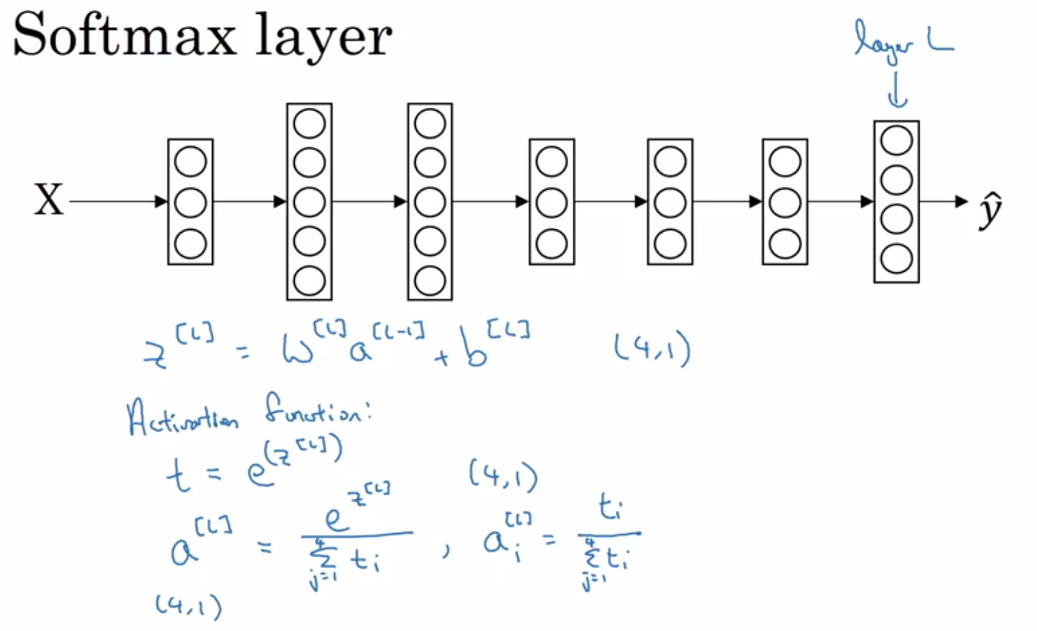
  • Softmax calculates the output probabilities of various classes using the formula: y_pred = exp(z_i) / sum_over_i ( exp(z_i) ).
  • Softmax outputs the probability distribution of the classes.
  • In hardmax, we assign one class as 1 and the others as 0.
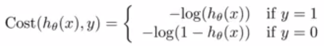
Cross Entropy:

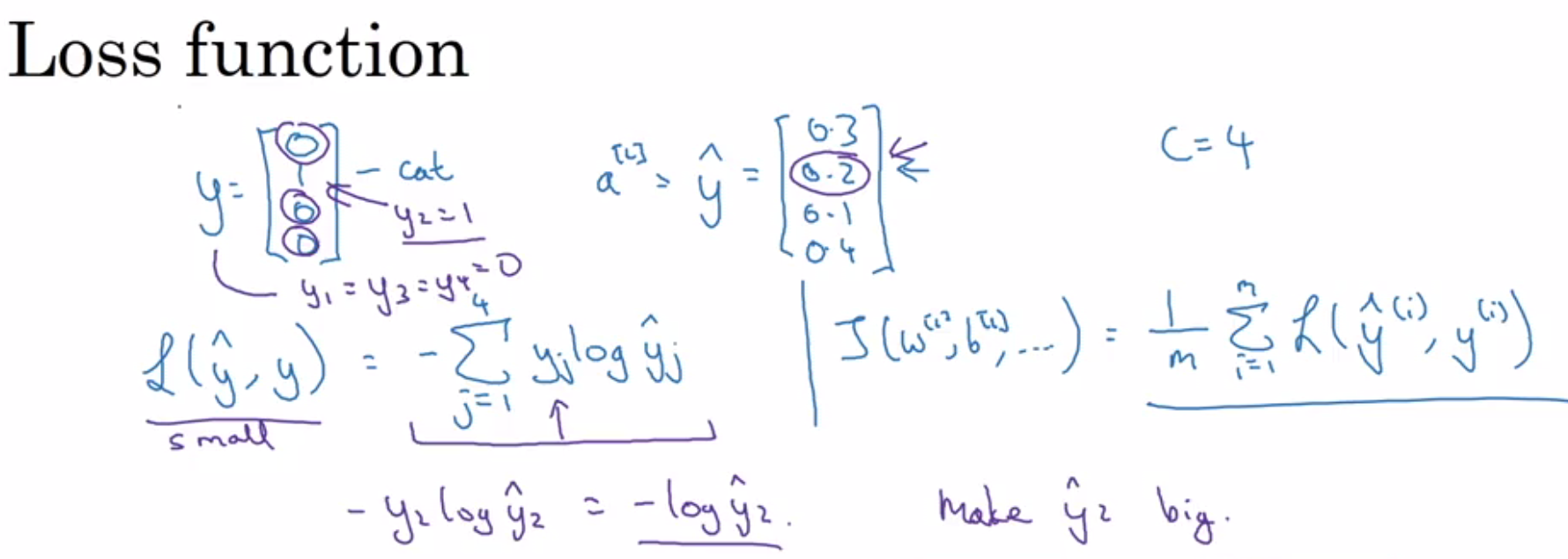
  • Cross entropy is a loss function commonly used in classification tasks.
  • The loss is calculated using the formula: Loss = - sum [y_actual * log(y_pred)].
  • For example, if the actual class is [1, 0, 0, 0, 0]:
    • y_pred_1 = [0.1, 0.5, 0.1, 0.1, 0.2]
    • y_pred_2 = [0.1, 0.6, 0.1, 0.1, 0.1]
  • The loss will be the same for y_pred_1 and y_pred_2.
  • This is a key feature of multiclass log loss: it rewards or penalizes the probabilities of correct classes only, and the value is independent of how the remaining probability is split between incorrect classes. [0]
  • Cross entropy is same as loss function of logistic regression, it is just that there are two classes.
8

References:

NN : Batch Norm and Softmax Regression

This post is a lecture summary of Week 3 of the deep learning course by Andrew N. G, available at https://www.coursera.org/learn/deep-neural-network/home/welcome.

Hyperparameter Tuning

  • When the number of parameters is large, random search is better than grid search.
  • Grid search is more useful when the number of parameters is small, as it is more systematic.
  • Not all hyperparameters are equally important.
  • Choosing between babysitting one model (“Panda” strategy) or training multiple models in parallel (“Caviar”) depends on the computational resources available.

Batch Normalization

  • Normalizing input features speeds up learning by making the contours more circular.
  • In practice, z[2] is normalized instead of a[2].
  • β and γ are introduced to allow for non-zero mean and non-unit variance.
    • Suppose you have sigmoid activation and you want larger variance to better exploit non-linearity
  • Different β and γ values are used for each layer.
  • In deep learning frameworks, batch normalization is often a single flag.
  • When using normalization, the bias term (b) has no effect and can be eliminated.

screen shot 2019-01-15 at 11.53.57 am

screen shot 2019-01-15 at 12.06.40 pm

  • Batch normalization speeds up training, limits distribution shifts of activation, provides more consistent data to later layers, and has a slight regularization effect.
  • Mean-variance scaling with different β and γ values for each mini-batch introduces noise similar to dropout, challenging later layers to not depend on a single feature.
  • Larger mini-batch sizes result in smaller regularization, but batch normalization is not primarily used for regularization.
  • During scoring, calculate µ and σ using exponentially weighted averages across mini-batches for each layer during training.
  • These averages are running averages and do not require much memory.
  • Use the above values for scoring.

Softmax Regression

  • Softmax regression is a generalization of logistic regression.
  • The output vector has dimensions (C, 1) and uses the “Softmax activation” function.
  • Softmax activation involves taking exponentials and normalizing the values.
softmax_layer
  • When C = 2, softmax reduces to logistic regression.
  • The loss function remains the same: cross-entropy loss.
  • Only one class will have an actual value of 1, following the maximum likelihood function.
loss_function
  • The gradient of the last layer is dz = ŷ – y.
backprop

Optimization for NN

Mini-batch Gradient Descent:

  • Mini-batch gradient descent exhibits oscillations during descent.
  • Choosing mini-batch size:
    • For small training sets (< 2k samples), it is advisable to use batch gradient descent.
    • For larger training sets, mini-batches of sizes such as 64, 128, 256, or 512 are commonly used.
  • Cross-validation helps in finding the right trade-off.
  • Batch gradient descent: More training time is dominated by the processing of a single duration.
  • Stochastic gradient descent: More training time is dominated by the number of iterations required for convergence.
    • Vectorization is lost in the case of stochastic gradient descent.

Exponentially Weighted Moving Averages:

  • Exponentially weighted moving averages are computed using the formulas:
    • Vₜ = 0.9 * Vₜ₋₁ + 0.1 * θₜ
    • Vₜ = β * Vₜ₋₁ + (1 – β) * θₜ
  • Averaging over roughly the last 10 days of temperature is achieved using the factor 1 / (1 – 0.9).
  • Bias correction is necessary to eliminate the bias introduced when initializing with v₀ = 0.
  • The bias correction formula is: Vₜ = (1 – βᵗ) * (β * Vₜ₋₁ + (1 – β) * θₜ)
bias_correction

Gradient Descent with Momentum:

  • Gradient descent with momentum enables slower learning on the vertical axis and faster learning on the horizontal axis.
  • In practice, bias correction is not used after around 10 iterations.
gradient_descent_with_momentum.png

RMSprop:

  • RMSprop is used to handle situations where some dw values can be large.
  • Adding epsilon for numerical stability helps prevent division by zero.
  • Notice is the dw^2 in the formula below
rmsprop

Adam Optimization:

  • Adam optimization, short for Adaptive Moment Estimation, is one of the algorithms that works well across domains.
  • Default values commonly used for β₁ (0.9), β₂ (0.999), and ε (10^-8)
adam

Learning Rate Decay:

  • 1 epoch refers to one pass through the entire data.
  • In the case of mini-batches, one epoch can involve multiple iterations.
  • Different formulas are used for learning rate decay
learning_rate_decay.png

Local Optima:

  • Most points with zero gradient are not local optima but rather saddle points, especially in high-dimensional spaces.
  • Local optima are generally not observed due to the high dimensionality.
  • Plateaus can be problematic, with very small gradients leading to slower learning.

Inverted Dropout

This post is a lecture summary of the deep learning course by Andrew N. G, available at https://www.coursera.org/learn/deep-neural-network/home/welcome.

During Training:

  • Neurons are dropped out by setting them to zero.
  • The activation is adjusted by dividing it with the keep probability.
  • The expected value of z[4] (as shown in the screenshot below) should not be altered.
inverted_dropout

During Scoring:

  • If “inverted dropout” is used, no additional steps are necessary.
  • Other dropout techniques may require some computations.

Intuition:

  • Dropping out neurons causes inputs to the unit to be randomly dropped.
  • This prevents the unit from relying too heavily on a single feature and encourages it to distribute weights across multiple features.
  • Different layers can have different keep probabilities.

Side Effect:

  • The cost function is not well defined.
  • It’s not possible to check if the cost is consistently decreasing every iteration.
  • A debugging tool is used to address this issue.

Solution:

  • First, verify that everything is functioning correctly without dropout.
  • Then, gradually introduce dropout.

———————————————————————–

Other Regularization Techniques

  • Data augmentation, such as horizontal flipping, random cropping, and transformations.
  • Early stopping: Stop training at a certain iteration (e.g., 7k instead of 10k) based on the error observed on the development set.

Downside

  • Balancing optimization and avoiding overfitting can be challenging.
  • Mixing both objectives requires careful consideration.

Advantage

  • Unlike L2 regularization, dropout does not necessitate trying different lambda values repeatedly.

Negative sampling in word2vec

In the precious post we talked about skipgram model.

https://datastoriesweb.wordpress.com/2018/01/31/word2vec-and-skip-gram-model/


Now let’s say we have 1000 words and 300 hidden units, we shall have 300,000 wights in both hidden and output unit, which are two many parameters.

Output label during training is one hot vector with 999 zeros and single 1. We randomly select 5 zeros and update weight for six words only. (5 zeros and single 1). The more frequent word is the highr the probability of it getting selected. Google paper has mentioned some emperical formula for this. This is know as negative sampling.

Above was for output layer. In hidden layer weights are updated only for input words. (Irrespective if it is negative sampling or not)


Reference:

http://mccormickml.com/2017/01/11/word2vec-tutorial-part-2-negative-sampling/


Word2Vec and skip gram model

Skip gram model

  • Weights of hidden layer serves as word vectors
  • There is just one hidden layer and one output layer(softmax)
  • Hidden layer does not have any activation
  • As input is one-hot vector, output is also one-hot vector
    • output of hidden layer would be corresponding word vector
  • In the below diagram:
    • Size of input (1 x 10000)
    • Size of output (1 x 10000)
    • Weight of hidden layer (10000 x 300)
    • Weight of output layer (300 x 10000)
    • So too many weight to learn – solution : negative sampling
  • Training pair would be nearby words in predefined window
    • We can imagine how huge can that be
    • It is pair of words both one-hot encoded
    • Sure, we need to know previously size of our vocabulary (which will be dimension of one-hot vector)
  • The paper google release was trained on google news data and used 300 dimension vector, which means 300 neuron in hidden unit. The paper lists this no and size of training words and efficiency.
    • Not there is one more parameter called named window size which was set to 5.
    • It means that 5 words before and after center words are considered as pair for training data.
  • There is no activation function on the hidden layer neurons, but the output neurons use softmax.
word2vec.PNG

Why word2vec

  • Earlier NLP methods used to rely on synonyms/hypernyms which is not totally contextual
    • Earlier case was mainly one hot encoding of vector
  • “proficient” is synonym of good only in some context
  • New words are getting added everyday
  • All words are one-hot encoded
    • Somewhat similar word might be orthagonal
    • Size of vector become too large

Role of TF-IDF

  • It is a scoring mechanism
  • Instead of average vectors of all the words in document we can have weighted average by TF-IDF score

There are two more things:

  • Continuous Bag Of Words
  • Negative sampling

CBOW

  • It also takes average of context words
    • One argument in the favour that averaging is valid
  • Both CBOW and skip gram does not add non-linearity in hidden layer
    • Output layer uses softmax
    • Idea is that word-embedding is used to predict target word.

References :

http://mccormickml.com/2016/04/19/word2vec-tutorial-the-skip-gram-model/

http://cs224d.stanford.edu/

http://web.stanford.edu/class/cs224n/syllabus.html

http://nadbordrozd.github.io/blog/2016/05/20/text-classification-with-word2vec/

Deep learning taking off

I recently started Andrew Ng’s specialization on deep learning and found these two interesting points :

One is about how performance of algorithm changes with the amount of data. Traditional algorithms have limits but Deep neural network has more advantages.

whyD


Also for the small amount of data traditional algorithms may win over neural nets with good feature engineering.

Second reason is that deep learning requires data, computation and efficient algorithms. Recent years have seen significant advancement in algorithm to increase computation efficiency. For example sigmoid to ReLU was an algorithmic change which allowed gradient to converge faster.


Ref : https://www.coursera.org/learn/neural-networks-deep-learning/home