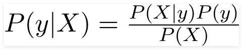
A probability model is an extension of Bayes’ rule. It makes two assumptions:
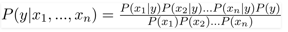
Independence of Features: This assumption assumes that all features are independent of each other. However, it does not hold true in many cases. For example, having higher temperature does not necessarily imply higher humidity.
Equal Weight of Features: This assumption assumes that all features have equal importance or weight in the model.
Classification Model
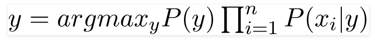
The classification model involves the following steps:
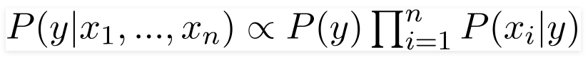
Probability of Each Class: P(y) represents the probability of each class based on the training set.
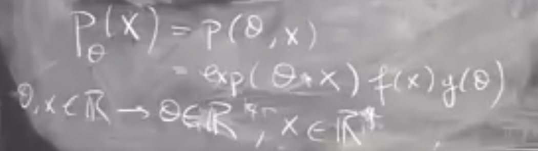
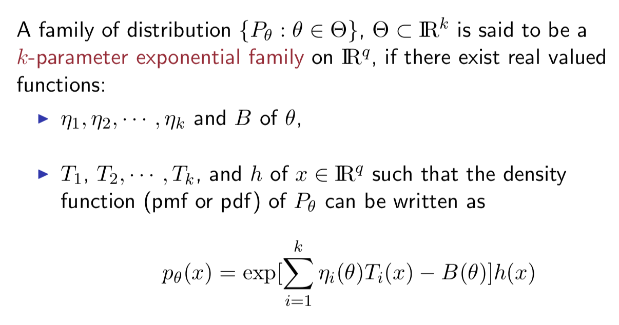
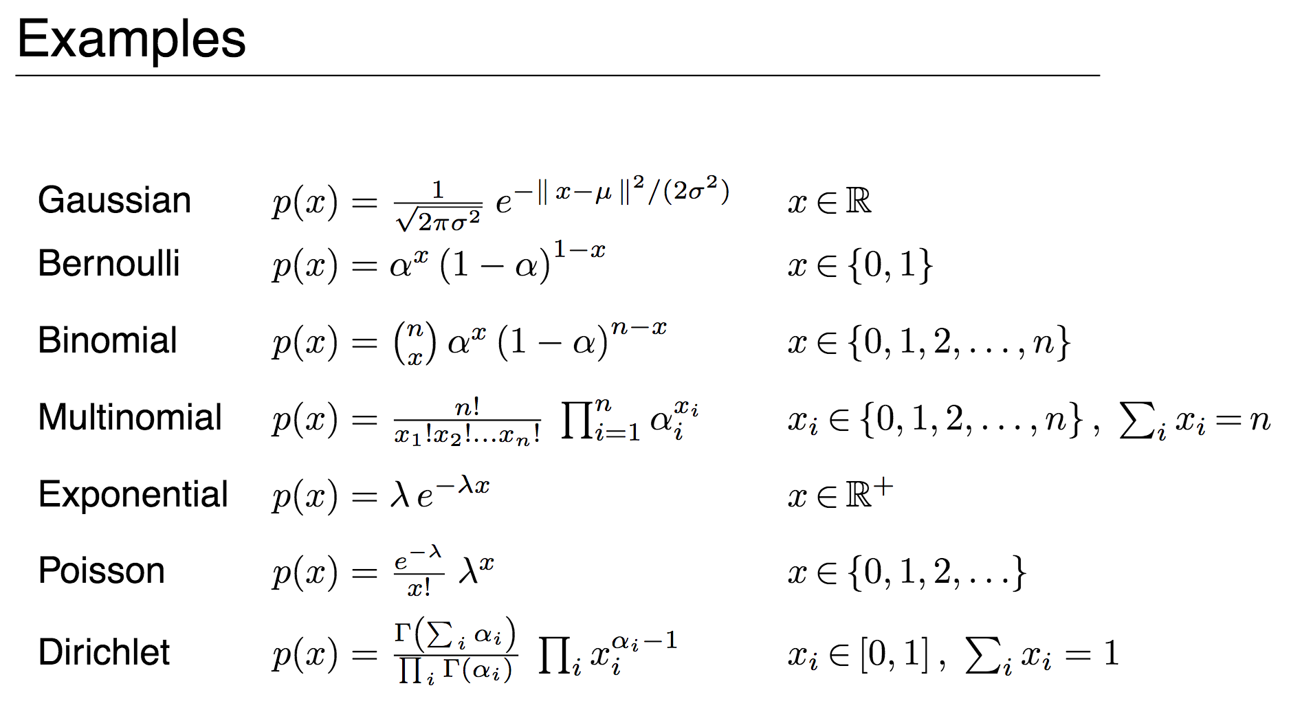
Probability Estimation of Feature Values: The goal is to estimate the probability distribution of each feature value given a specific class, denoted as P(x_i|y). For discrete features, this can be achieved through simple probability calculations, such as multinomial Naive Bayes. For continuous features, Gaussian distributions can be used. In the case of count data, multinomial distributions are suitable.
Parameter Estimation: Parameter estimation is performed for each combination of class and feature.
Scikit-learn and Distribution Types: Scikit-learn library provides implementations of Gaussian Naive Bayes, Bernoulli Naive Bayes, and multinomial Naive Bayes classifiers. These classifiers refer to the distribution of features. It is important to note that different features can follow different distributions. Therefore, customization of the distribution based on the application may be necessary.
Advantages
Fast and Easy Implementation: Naive Bayes classifiers are known for their simplicity and efficiency in implementation.
Acceptable Classification Performance: While Naive Bayes classifiers may not always accurately predict probabilities, their classification performance is generally satisfactory.
Disadvantage
Independence Assumption: The assumption of feature independence does not hold true in all scenarios, which can affect the model’s accuracy.
Thompson sampling is one approach for Multi Armed Bandits problem and about the Exploration-Exploitation dilemma faced in reinforcement learning. It is also know as posterior sampling.
Challenge in solving such a problem is that we might end up fetching the same arm again and again. Bayesian approach helps us solving this dilemma by setting prior with somewhat high variance.
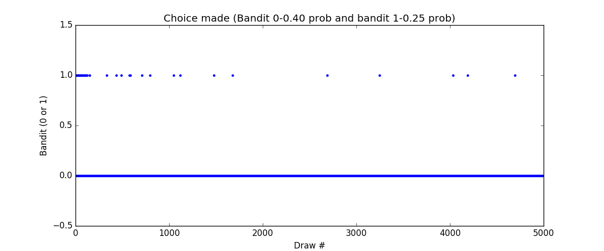
Here is the code for two armed bandit. One has success probability of 40% (bandit 0) and another has 25% (bandit 1).
We are using beta distribution for deciding which arm to pull. Beta distribution has two parameter alpha and beta. Higher values of alpha, pulls distribution towards 1. Beta distribution is always confined between 0 and 1.
How we train is that for each feedback we receive we increment alpha by 1 if it was success or beta by 1 in case of failure. For choosing the arm we draw random sample from the distribution of each arm and select the arm with highest value.
This file contains hidden or bidirectional Unicode text that may be interpreted or compiled differently than what appears below. To review, open the file in an editor that reveals hidden Unicode characters.
Learn more about bidirectional Unicode characters
And here is simulation results. We see that initially both the the armed are pulled frequently but slowly arm 1 is pulled less and less, but it is never straight away zero.
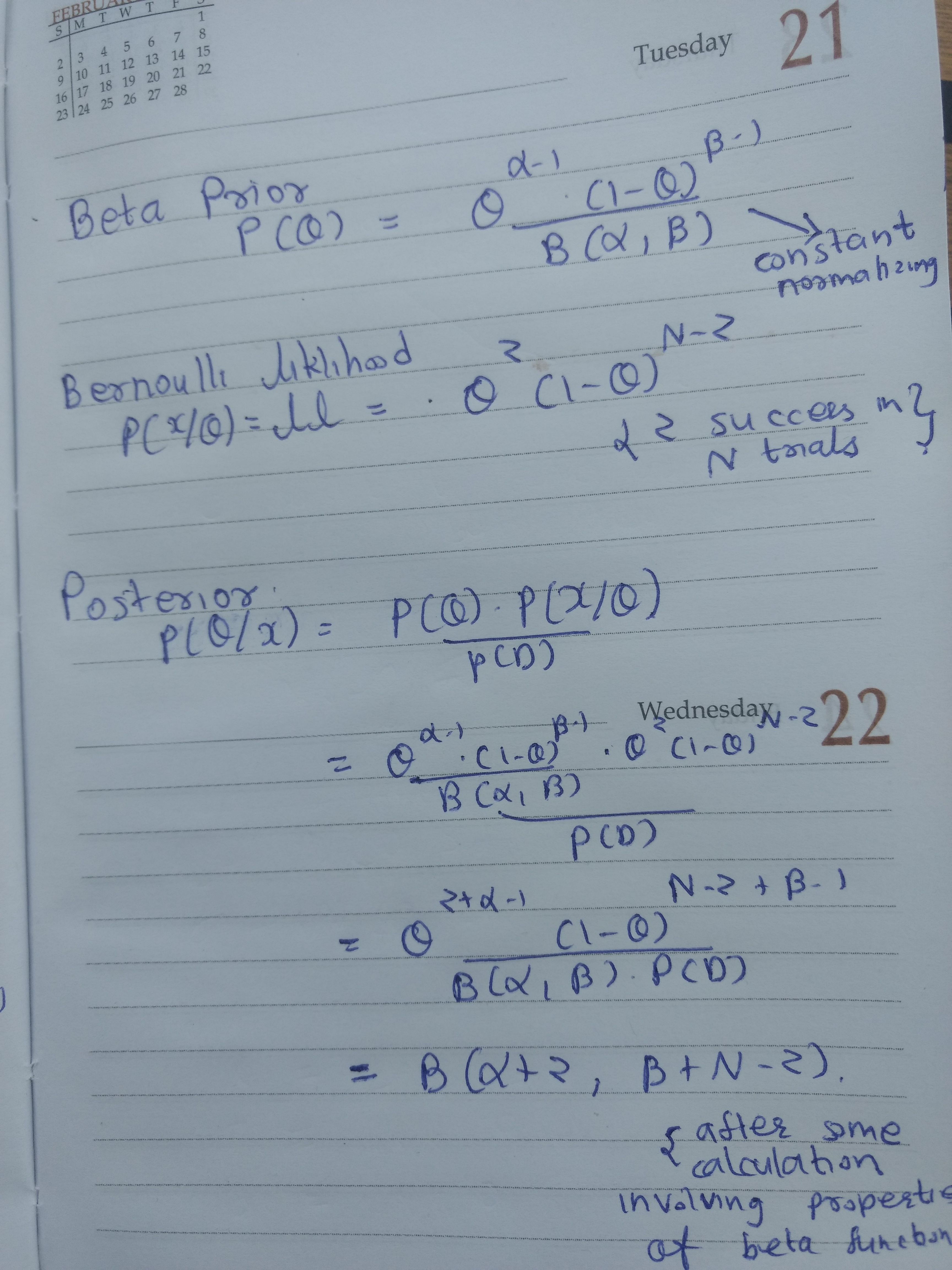
Math Behind Increasing alpha and beta
In one line posterior is beta distribution for beta prior and Bernoulli likelihood. In other words beta is a conjugate prior for Bernoulli likelihood. List of various conjugate prior is available at [1].
PDF of beta distribution is simple once you think in terms of the effect of alpha and beta.
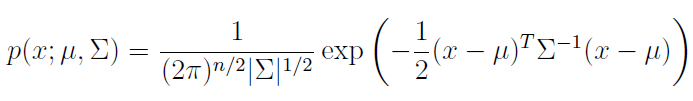
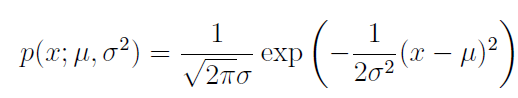
Look at note below, formula of beta distribution is not complex, actually it is very similar to
Σ being a positive definite ensure quadratic bowl is downwards
σ2 also being positive ensure that parabola is downwards
On Covariance Matrix
Definition of covariance between two vectors:
When we have more than two variable we present them in matrix form. So covariance matrix will look like
Above is very similar to how we compute sigma^2 in 1-D = (x – mu)^2
Formula of multivariate gaussian distribution demands Σ to be singular and symmetric positive semidefinite, which in terms means sigma will be symmetric positive semidefinite.
For some data above demands might not meet
Side Note
Covariance is directional measure
Correlation is scaled measure
We normalise by individual variance
Derivations
Following derivations are available at [0]:
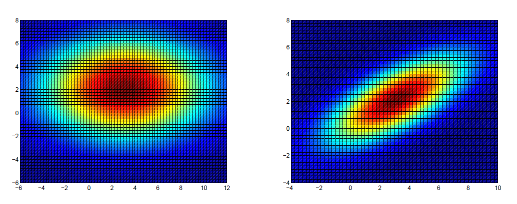
We can prove[0] that when covariance matrix is diagonal (i.e there is variables are independent) multivariate gaussian distribution is simply multiplication of single gaussian distribution of each variable.
It was derived that shape of isocontours (figure 1) is elliptical and axis length is proportional to individual variance of that variable
Above is true even when covariance matrix is not diagonal and for dimension n>2 (ellipsoids)
First part above says that bi-variant destitution can be generated from two standard normal distribution z = N(0,1).
For any given k-variant Gaussian we can represent it as linear combination of k standard normal distribution. One simpler way to find these coefficient is Cholesky decomposition. Theorem 1 below stats the same thing.
This has a reference from [1].
Linear Transformation Interpretation
This was proved in two steps [0]:
Step-1 : Factorizing covariance matrix
Step-2 : Change of variables, which we apply to density function
On Practical Example
Height, wight and waist size of men in US (Of course it weight can be negative, so it is approximately normal)
Understanding probability rules and solving tricky probability questions can be challenging. In this blog post, we will explore key probability rules and discuss solutions to some intriguing questions.
Probability Rules:
Joint Distribution: The probability of events X and Y occurring together is denoted as p(X, Y) and is known as the joint distribution.
Conditional Distribution: The probability of event X given event Y is denoted as p(X/Y) and is known as the conditional distribution.
Marginal Distribution: The probability of event X, with event Y marginalized out, is denoted as p(X) and is known as the marginal distribution.
Operations:
Making Conditional Distribution: To obtain the conditional distribution, normalization is required.
Marginalization: Marginalization does not require normalization.
Note: It is not possible to derive the conditional distribution from the joint distribution solely through integration. There is no direct relationship between them.
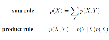
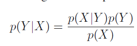
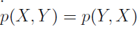
There are just two rules for probability. Sum rule and product rules. And then there is Bayes theorem. Bayes theorem can be derived from product rule and the fact that P(x,y) = P(y,x)
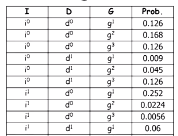
We might want to look at a table like below and calculate joint and conditional distribution and marginalized out one of the variable. [1]
Probability Tricky Question
This questions are taken from [2]. One key to solve this question is write down the sample space and keep eliminating choices. Don’t conclude in hurry.
Q1 : A man comes up to you on the street and says: I have two children. At least one of them is a boy. What is the probability that the other child is also a boy?
Q2 : I have two kids, what are the odds I have 2 boys?
Q3 : A man comes up to you on the street and says: I have two children. The older one is a boy. What is the probability that the other child is also a boy?
Q4 : A man comes up to you on the street and says: I have two children. One is the boy standing here next to me. What is the probability that the other child is also a boy?
Q5 : Q. A man comes up to you on the street and says: I have two children. One of them is a boy who was born in the summer. What is the probability that the other child is also a boy? (There are four seasons : spring, summer, fall, winter)[0]
Ans1 : (1/3)
P(BG) is 1/2 and p(BB) = 1/4 in the universe
Ans2 : (1/4)
Ans3 : (1/2)
Ans4 : (1/2)
Ans5 : (7/15) [0]
Compare Q1 and Q5. Odd increases. Being born in summer is rare thing. If that rare thing has occurred there are higher chances of having two boys.
A bag contains (x) one rupee coins and (y) 50 paise coins. Four coins are taken from the bag and put away. If a coin is now taken at random from the bag, what is the probability that it is a one rupee coin?
Ans is x/(x+y). It will remain same if we take either 1/2/3/4/5 coins because we don’t know which coin has been withdrawn. It is like trying out all possibilities and when we sum, it would come out as 1 only. [4]
The probability of a car passing a certain intersection in a 20 minute windows is 0.9. What is the probability of a car passing the intersection in a 5 minute window? (Assuming a constant probability throughout)
Ans : 0.4377 [5]
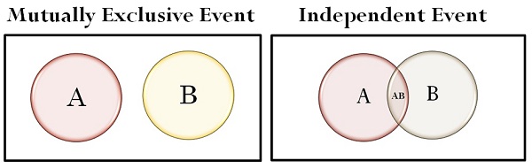
Independent Events
Mutually exclusive events means dependent event
For independent event = P(A/B) = P(A)
For mutually exclusive event if we know B has occurred, A will never occur.
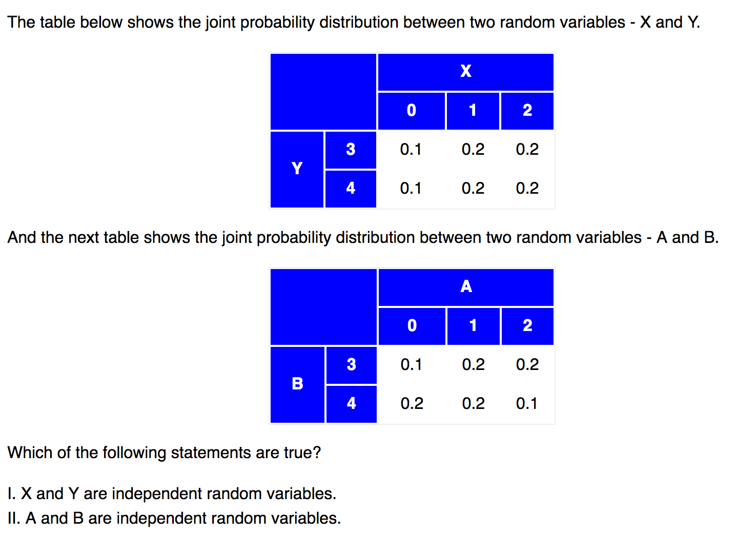
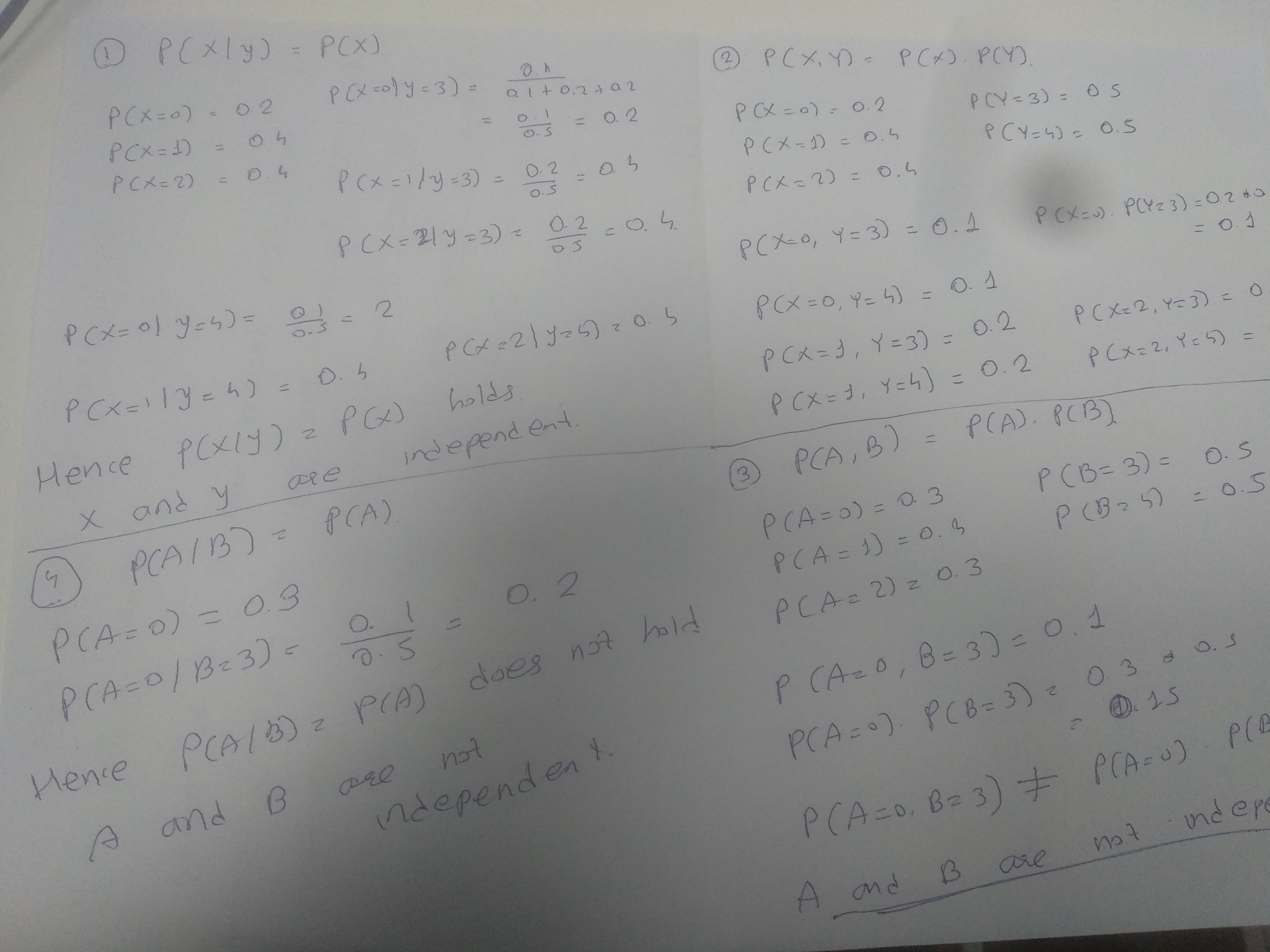
If two random variables, X and Y, are independent, they satisfy the following conditions.
P(x|y) = P(x), for all values of X and Y.
P(X, Y) = P(x ∩ y) = P(x) * P(y), for all values of X and Y.
Here is an example from [6]. Ans is that X and Y are independent, A and B are not.