Negative sampling in word2vec

In the precious post we talked about skipgram model.

https://datastoriesweb.wordpress.com/2018/01/31/word2vec-and-skip-gram-model/


Now let’s say we have 1000 words and 300 hidden units, we shall have 300,000 wights in both hidden and output unit, which are two many parameters.

Output label during training is one hot vector with 999 zeros and single 1. We randomly select 5 zeros and update weight for six words only. (5 zeros and single 1). The more frequent word is the highr the probability of it getting selected. Google paper has mentioned some emperical formula for this. This is know as negative sampling.

Above was for output layer. In hidden layer weights are updated only for input words. (Irrespective if it is negative sampling or not)


Reference:

http://mccormickml.com/2017/01/11/word2vec-tutorial-part-2-negative-sampling/


Derivation of backpropogation

Quick Summary:
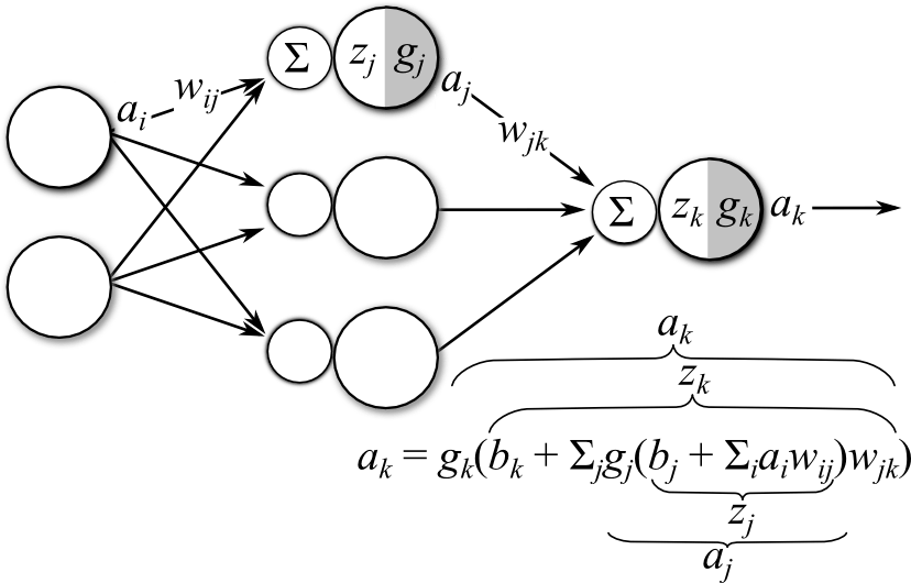


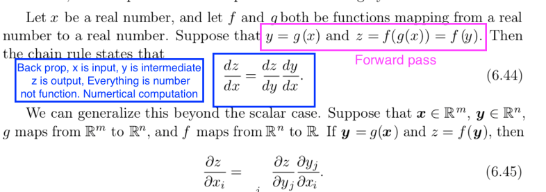
back_prop


Detailed Derivation:


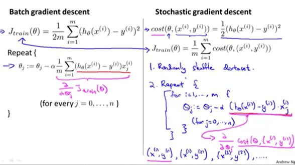
Even if you look at gradient descent below, error is multiplied by previous value. When input is higher it’s contribution to error is higher and will needs to change more.
gd


import numpy as np
# 1. Activation and Loss Functions
def relu(x):
return np.maximum(0, x)
def relu_derivative(x):
return (x > 0).astype(float)
def softmax_and_cross_entropy_loss(logits, y_true):
"""
Computes stable softmax and categorical cross-entropy loss together.
logits: (batch_size, num_classes)
y_true: (batch_size, num_classes) - One-hot encoded labels
"""
# Log-Sum-Exp trick for numerical stability
shifted_logits = logits - np.max(logits, axis=1, keepdims=True)
exps = np.exp(shifted_logits)
softmax_probs = exps / np.sum(exps, axis=1, keepdims=True)
# Compute Cross-Entropy Loss
batch_size = logits.shape[0]
# Add a tiny epsilon to prevent log(0)
loss = -np.sum(y_true * np.log(softmax_probs + 1e-15)) / batch_size
# The gradient of loss with respect to logits simplifies beautifully to: (probs - target)
d_logits = (softmax_probs - y_true) / batch_size
return loss, d_logits
# 2. Network Initialization
np.random.seed(42) # For reproducible results
input_dim = 3 # e.g., 3 features
hidden_dim = 4 # 4 neurons in the hidden layer
output_dim = 2 # 2 classes (Binary/Multiclass)
# Xavier/Glorot Initialization for weights
W1 = np.random.randn(input_dim, hidden_dim) * np.sqrt(2.0 / input_dim)
b1 = np.zeros((1, hidden_dim))
W2 = np.random.randn(hidden_dim, output_dim) * np.sqrt(2.0 / hidden_dim)
b2 = np.zeros((1, output_dim))
# Dummy Training Data (Batch of 2 samples)
X = np.array([[0.5, -0.2, 0.1],
[0.1, 0.8, -0.5]])
# One-hot encoded true targets
Y = np.array([[1.0, 0.0], # Class 0 is correct
[0.0, 1.0]]) # Class 1 is correct
learning_rate = 0.1
# 3. Training Iteration (Forward & Backward Pass)
for epoch in range(3):
# --- FORWARD PASS ---
# Hidden Layer
z1 = np.dot(X, W1) + b1
a1 = relu(z1)
# Output Layer (Generates Raw Logits)
logits = np.dot(a1, W2) + b2
# Compute Loss and the gradient at the final layer
loss, d_logits = softmax_and_cross_entropy_loss(logits, Y)
# --- BACKWARD PASS (Backpropagation) ---
# Gradients for Output Layer weights and biases
dW2 = np.dot(a1.T, d_logits)
db2 = np.sum(d_logits, axis=0, keepdims=True)
# Gradient flowing back into the hidden layer
da1 = np.dot(d_logits, W2.T)
dz1 = da1 * relu_derivative(z1) # Backprop through ReLU
# Gradients for Hidden Layer weights and biases
dW1 = np.dot(X.T, dz1)
db1 = np.sum(dz1, axis=0, keepdims=True)
# --- GRADIENT DESCENT ---
W2 -= learning_rate * dW2
b2 -= learning_rate * db2
W1 -= learning_rate * dW1
b1 -= learning_rate * db1
print(f"Epoch {epoch+1} - Loss: {loss:.4f} | Raw Logits Sample 1: {logits[0]}")