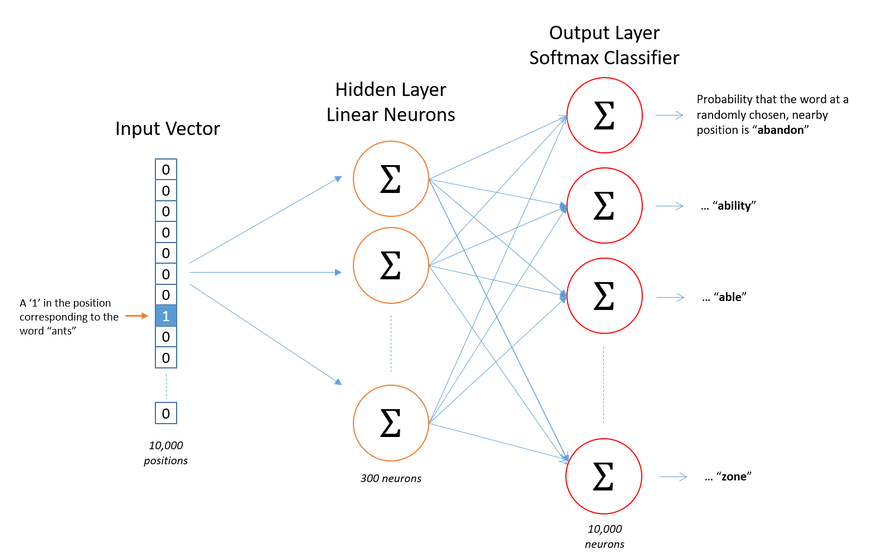
Now let’s say we have 1000 words and 300 hidden units, we shall have 300,000 wights in both hidden and output unit, which are two many parameters.
Output label during training is one hot vector with 999 zeros and single 1. We randomly select 5 zeros and update weight for six words only. (5 zeros and single 1). The more frequent word is the highr the probability of it getting selected. Google paper has mentioned some emperical formula for this. This is know as negative sampling.
Above was for output layer. In hidden layer weights are updated only for input words. (Irrespective if it is negative sampling or not)
Training pair would be nearby words in predefined window
We can imagine how huge can that be
It is pair of words both one-hot encoded
Sure, we need to know previously size of our vocabulary (which will be dimension of one-hot vector)
The paper google release was trained on google news data and used 300 dimension vector, which means 300 neuron in hidden unit. The paper lists this no and size of training words and efficiency.
Not there is one more parameter called named window size which was set to 5.
It means that 5 words before and after center words are considered as pair for training data.
There is no activation function on the hidden layer neurons, but the output neurons use softmax.
Why word2vec
Earlier NLP methods used to rely on synonyms/hypernyms which is not totally contextual
Earlier case was mainly one hot encoding of vector
“proficient” is synonym of good only in some context
New words are getting added everyday
All words are one-hot encoded
Somewhat similar word might be orthagonal
Size of vector become too large
Role of TF-IDF
It is a scoring mechanism
Instead of average vectors of all the words in document we can have weighted average by TF-IDF score
There are two more things:
Continuous Bag Of Words
Negative sampling
CBOW
It also takes average of context words
One argument in the favour that averaging is valid
Both CBOW and skip gram does not add non-linearity in hidden layer
Output layer uses softmax
Idea is that word-embedding is used to predict target word.
From Matmul to Embedding tables
When you train a Word2Vec model, you are fundamentally initializing and training embedding tables using the Word2Vec objective function.
How Word2Vec Uses Embedding Tables
In standard Word2Vec (specifically the Skip-gram architecture), the model maintains two separate embedding tablesfor the entire vocabulary:
[ Vocabulary Size (V) ]
/ \
/ \
1. Target Embedding Table 2. Context Embedding Table
(Shape: V x Dimension) (Shape: V x Dimension)
Target Table ($\mathbf{W}$): Used when a word acts as the “center” or target word.
Context Table ($\mathbf{W}’$): Used when a word appears in the surrounding window of a target word.
Step-by-Step Mechanics of Training
When the model processes a sentence chunk like “the dog barks”, where dog is the target word and barks is the context word:
The Lookup: The unique integer ID for “dog” is used to look up a vector from the Target Table. The ID for “barks” looks up a vector from the Context Table.
The Comparison: The model takes the dot product of these two vectors to measure how “close” they are in vector space.
The Loss & Update:
If using Negative Sampling, the model also pulls random “noise” words from the Context Table (like “banana”).
It calculates the loss (maximizing the dot product for “barks”, minimizing it for “banana”).
Backpropagation updates the specific rows in both embedding tables for those words.
The Final Output
Once training is complete, the Context Table is discarded, and the Target Embedding Table becomes your final dictionary of word vectors.
Original paper
We are revving activation and using matul to calculate dot products
On the hidden layer. The paper’s architecture is:
one-hot (V) → W_in (V×d) → h (d) → W_out (d×V) → scores (V) → loss
That middle h is drawn as a layer, so it looks like an MLP with one hidden layer. But there’s no activation on it. h is literally the row of W_in you just looked up — no ReLU, no tanh, nothing. Mikolov’s phrase for it in the paper is that the nonlinear hidden layer is removed; that’s the stated reason the model trains fast enough to run on billions of words.
PyTorch Implementation
class SkipGramNS(nn.Module):
def __init__(self, V, d):
super().__init__()
self.emb_in = nn.Embedding(V, d) # center vectors (the ones you keep)
1. Softmax makes words compete; contexts shouldn’t compete.
A center word like cat has many valid contexts: sat, the, chased, animal. Softmax normalizes across all of them, so probability is a fixed budget — pushing sat up necessarily pushes chased down, even though both are correct. Binary cross-entropy scores each pair on its own: “is this pair real, yes or no.” Every genuine context can score high at the same time. The problem is really multi-label, and BCE treats it that way.
2. Sampled softmax needs a correction term; negative sampling doesn’t.
To make sampled softmax approximate the true softmax, you have to subtract log(k · q(w)) from each logit, where q(w) is the probability you sampled that word. Without it you’re biased — frequent words get sampled more often and get systematically over-penalized. That means you must track your sampling distribution and plumb it into the loss. Negative sampling just drops that term and accepts that it’s a different objective.
3. Word2vec never needs the probability.
Sampled softmax exists to give you a usable estimate of p(context | center). Word2vec throws the scores away and keeps the embedding table. If you don’t need a calibrated distribution, you don’t need the machinery that produces one.
The honest caveat: this ordering flips in modern retrieval. Two-tower recommender systems mostly use sampled softmax with the logQ correction rather than BCE, because ranking quality against a large corpus is exactly the case where the normalization helps and the popularity bias hurts. So “negative sampling is better” is a word2vec-specific claim, not a general one.