Some people use term bagging and boosting, some use parallel and sequential ensembles. I have written a post on AdaBoost previously. So we are familiar with boosting idea.
In AdaBoost we had a formula for generating labels (label/sample weight in loss function to be precise) for next iteration. In gradient boosting we fit gradient of loss function with respect to predictions.
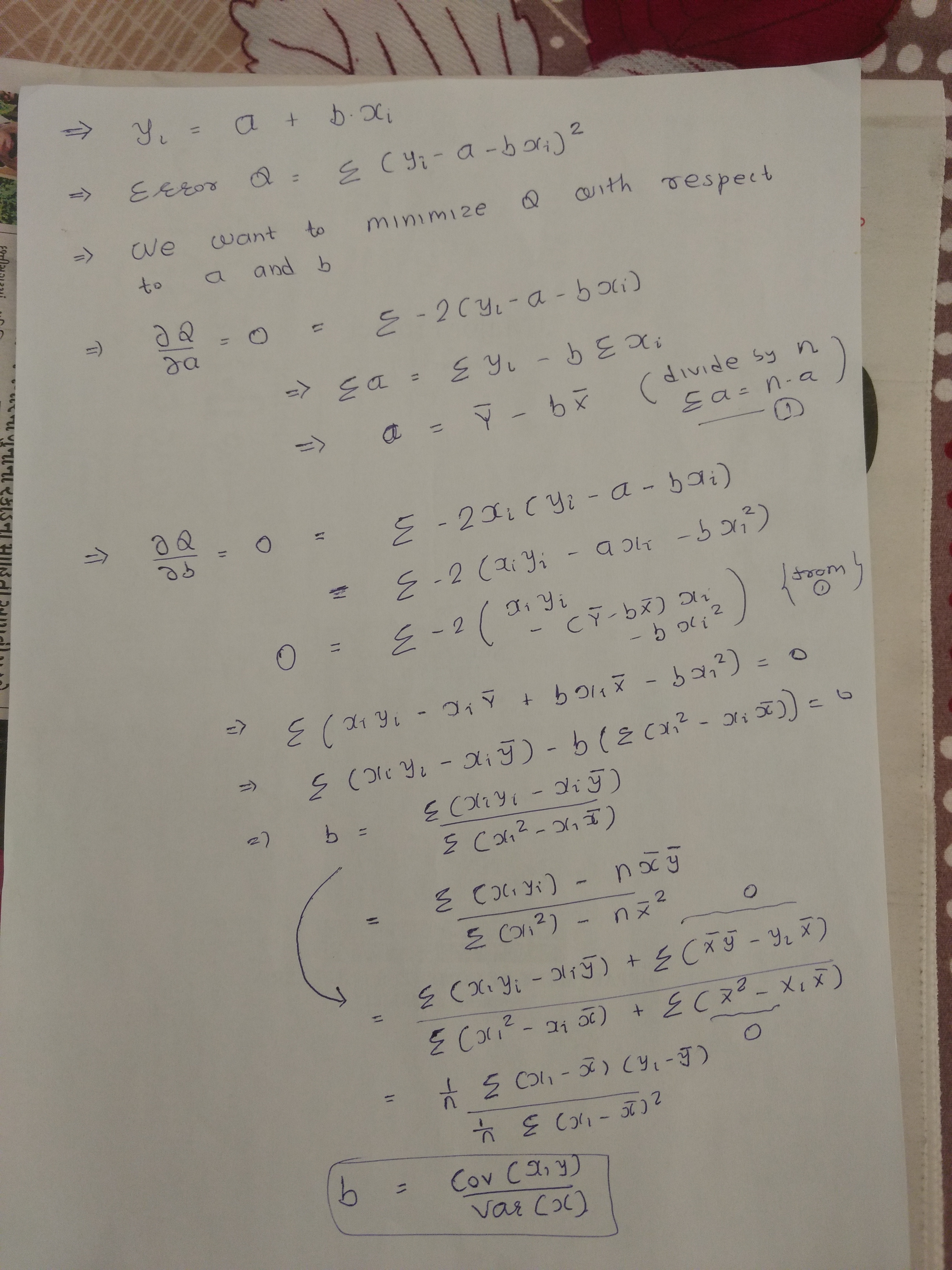
Prof Balaraman notes
- Most of this post contains info from [0]. However Prof. Balaraman offers intuitive perspective in one of his lectures. [3]
- My handwritten note on that is available at [2]
- We can write decision tree as equation where regions and value in the region are parameters.
- Two steps of gradient boosting
- Fit gradient of loss function using regression trees (least square loss)
- Compute values in region using loss defined for application (ndcg for ranking, log-loss for classifier anything)
- Whatever is application loss, we fit regression tree using least square
- Parametric gradient descent can be seen as series of summation starting from initial guess.
- Related paper [4]
Basis Functions
- Basis functions
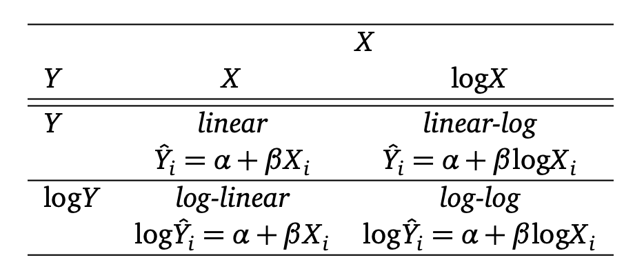
- If we want to fit non linear curve with simple linear regression, we will create polynomial features
- It is not limited to regression though
- Adaptive Basis function
- Instead of we defining above functions, we learn them
- This can be framed as optimisation problem and can be solved by gradient descent/newton’s method for some hypothesis space
- How to include Tree’s in base hypothesis space
- Something which we can not differentiate
- Even if we fix parameters to split on output is still not continuous
- So it is difficult
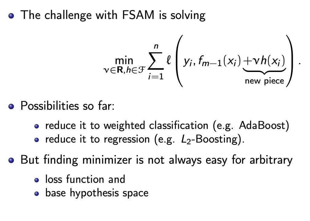
FSAM
- FSAM
- Forward Stage-wise Additive Modelling
- AdaBoost is example of this, another example is L2 boosting
- We can say weak function is step direction and coefficient is step size
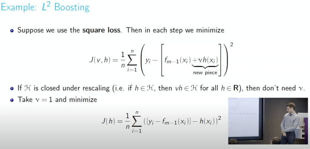
- L2 Boosting also example of FSAM
- We are fitting residual
- To prevent overfitting we can reduce step size
- If v*h(x) is also in H, we can remove v. (closed under rescaling)
- h(x) can be decision stump we can keep going as long as residuals exist (It will certainly overfit after few iterations)
- Adaboost
- It works for classification problem
- When the loss function in FSAM is exponential loss of margin, it reduces adaboost
- margin = y*f(x)
- We had encountered that in SVM
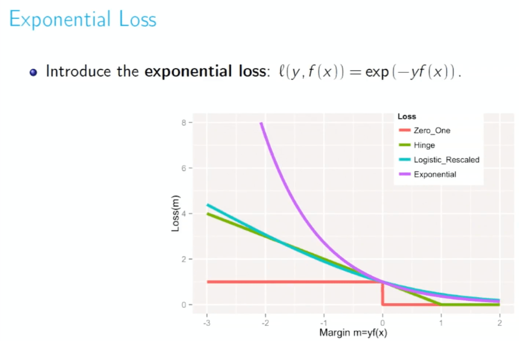
- Disadvantages of AdaBoost
- Gives too much penalty for negative margin, look at the curve of exponential above
- Mislabel training data
- Sometimes there is noise in world
- Does not work when there is high baye’s error
- Also it seems AdaBoost formulation is very much tied to classification
- We probably needs to tweak it to apply it to ranking problem
- But gradient boosting can be applied to any problem (loss function)
- Because Tree is alway using L2 loss
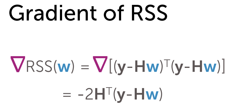
Functional Gradient Descent
- Gradient is pseudo residuals
- For L2 loss it is actually residuals (difference between y and f)
- Examples where residuals are not just difference between y and f
- logistic loss
- ranking using ndcg
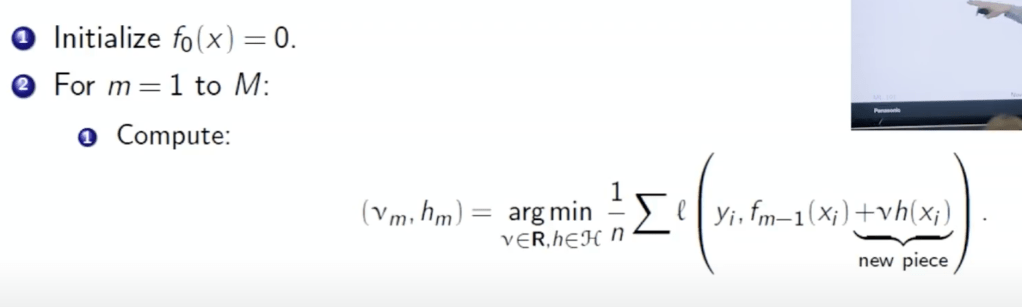
- We fit this gradient(pseudo-residuals) with weak function
- Regression Tree is most common
- We find closest approximation to gradient step in base hypothesis space (which is functional space)
- Here we minimize square loss (regression problem)
- Earlier tree used to be just stumps
- That is num of leaf node = 2
- Now a days xgboost/light gbm takes upto 8/16 leaf nodes as well
- Note that while calculating gradient the hypothesis function is not involved anywhere
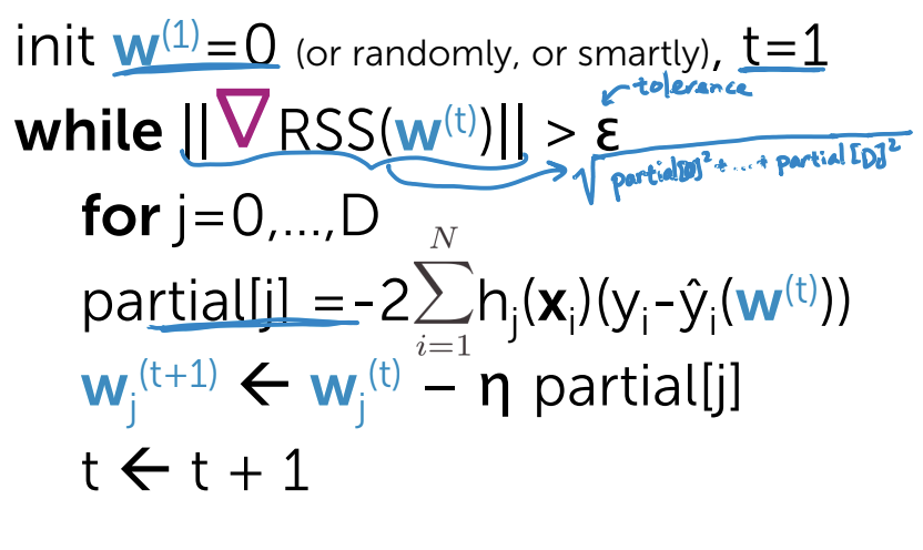
- How do we calculate gradient over function space
- In close form expression it might look complicated
- From numerical computation perspective we need gradient at just one point (of dimension training data size)
- This is just like taking gradient of weights in linear regression
- Here size of gradient vector would be number of training examples
- In most of the method we take gradient of parameters, here we are taking gradient of predictions
- What should be step size
- Line search
- Regularisation parameter (similar to what we use for any gradient based optimisation)
- This is more common
Reference
[0] https://www.youtube.com/watch?v=fz1H03ZKvLM
[1] https://davidrosenberg.github.io/mlcourse/Archive/2016/Lectures/8b.gradient-boosting.pdf
[2] https://github.com/arcarchit/datastories/blob/master/notes/gradient_boost_iitm.pdf