Optimization for NN

Mini-batch Gradient Descent:

  • Mini-batch gradient descent exhibits oscillations during descent.
  • Choosing mini-batch size:
    • For small training sets (< 2k samples), it is advisable to use batch gradient descent.
    • For larger training sets, mini-batches of sizes such as 64, 128, 256, or 512 are commonly used.
  • Cross-validation helps in finding the right trade-off.
  • Batch gradient descent: More training time is dominated by the processing of a single duration.
  • Stochastic gradient descent: More training time is dominated by the number of iterations required for convergence.
    • Vectorization is lost in the case of stochastic gradient descent.

Exponentially Weighted Moving Averages:

  • Exponentially weighted moving averages are computed using the formulas:
    • Vₜ = 0.9 * Vₜ₋₁ + 0.1 * θₜ
    • Vₜ = β * Vₜ₋₁ + (1 – β) * θₜ
  • Averaging over roughly the last 10 days of temperature is achieved using the factor 1 / (1 – 0.9).
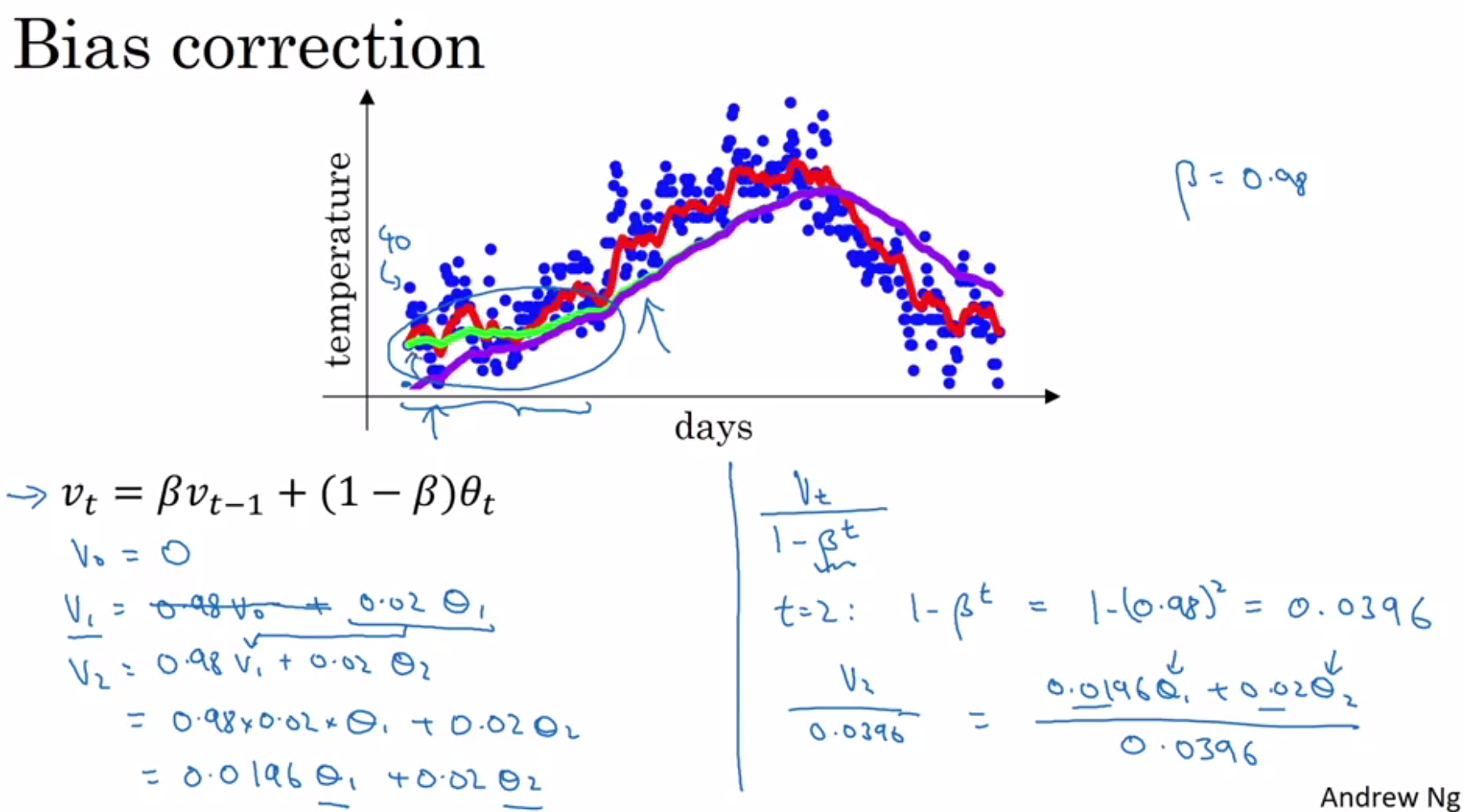
  • Bias correction is necessary to eliminate the bias introduced when initializing with v₀ = 0.
  • The bias correction formula is: Vₜ = (1 – βᵗ) * (β * Vₜ₋₁ + (1 – β) * θₜ)
bias_correction

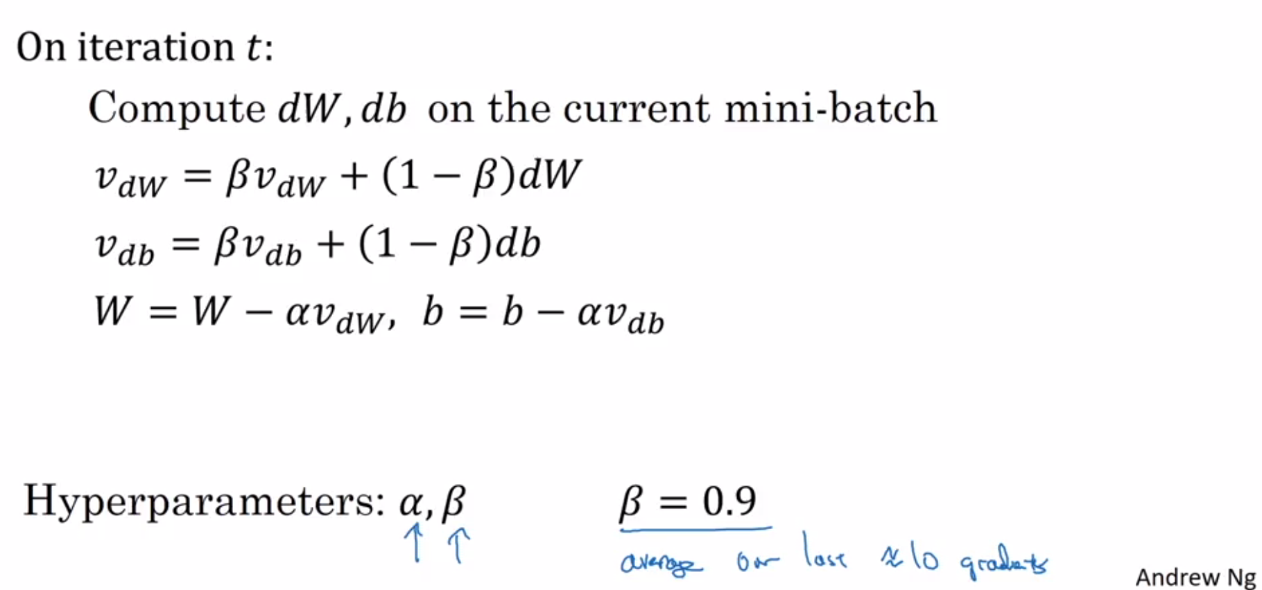
Gradient Descent with Momentum:

  • Gradient descent with momentum enables slower learning on the vertical axis and faster learning on the horizontal axis.
  • In practice, bias correction is not used after around 10 iterations.
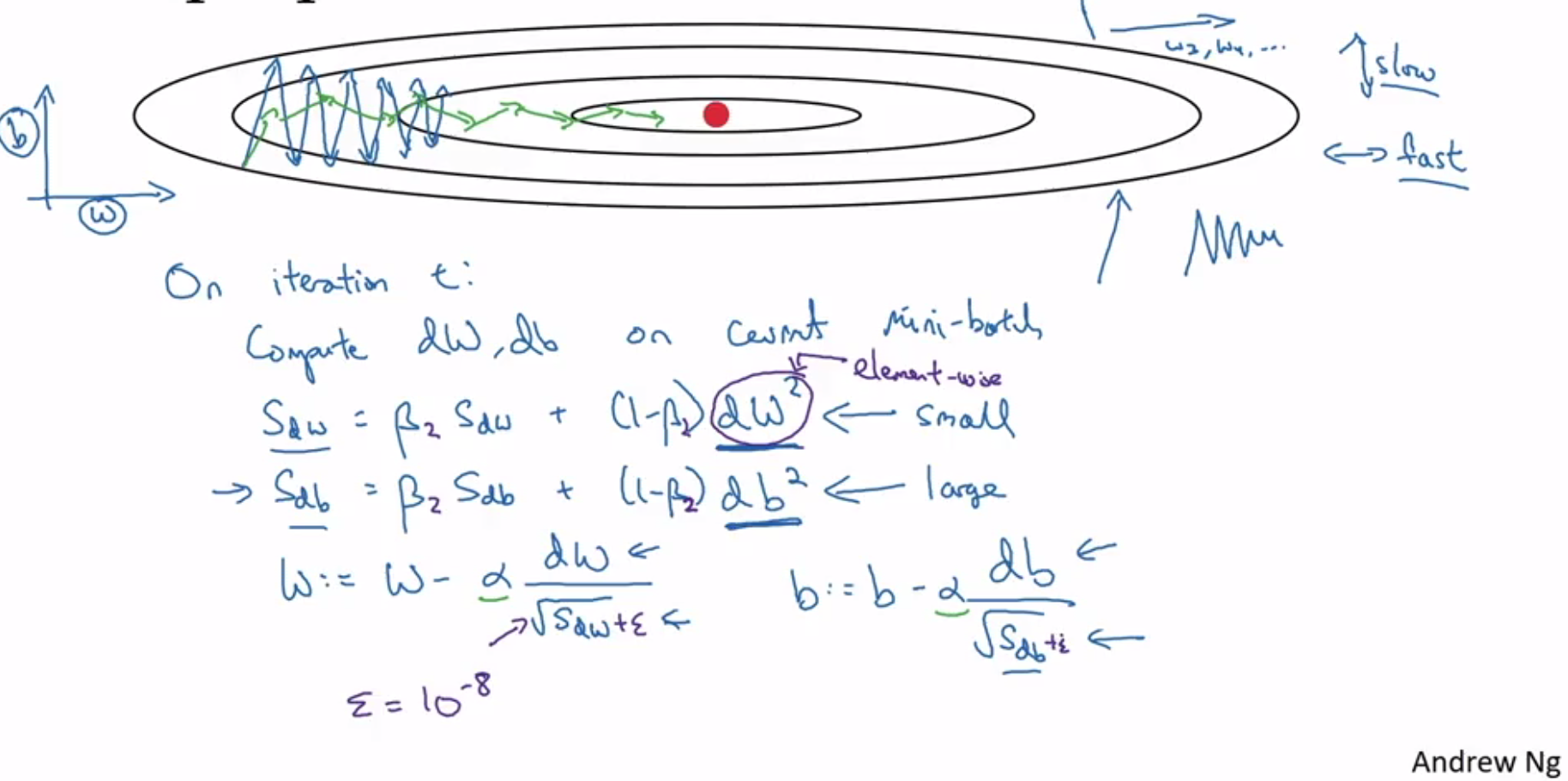
gradient_descent_with_momentum.png

RMSprop:

  • RMSprop is used to handle situations where some dw values can be large.
  • Adding epsilon for numerical stability helps prevent division by zero.
  • Notice is the dw^2 in the formula below
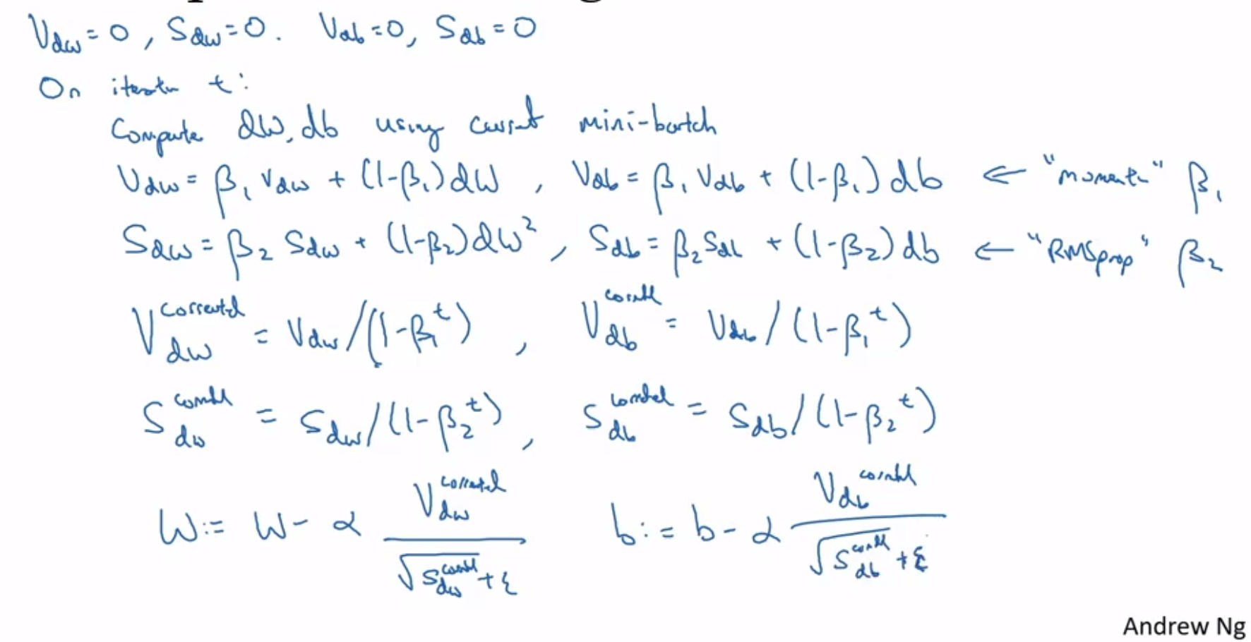
rmsprop

Adam Optimization:

  • Adam optimization, short for Adaptive Moment Estimation, is one of the algorithms that works well across domains.
  • Default values commonly used for β₁ (0.9), β₂ (0.999), and ε (10^-8)
adam

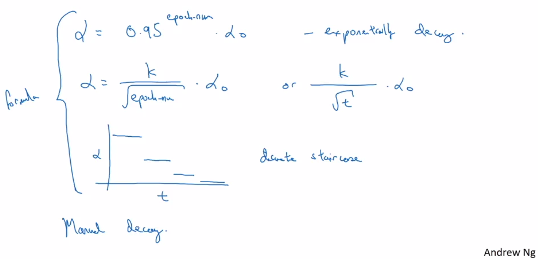
Learning Rate Decay:

  • 1 epoch refers to one pass through the entire data.
  • In the case of mini-batches, one epoch can involve multiple iterations.
  • Different formulas are used for learning rate decay
learning_rate_decay.png

Local Optima:

  • Most points with zero gradient are not local optima but rather saddle points, especially in high-dimensional spaces.
  • Local optima are generally not observed due to the high dimensionality.
  • Plateaus can be problematic, with very small gradients leading to slower learning.

Step Size in Descent Methods

Descent Method

general_descent

  • When the descent direction is opposite to gradient is is called gradient descent.
  • We also have steepest descent and newton’s algorithm
  • In this post we will focus on line search
  • Term is called ‘line search’ because step size t determines where along the line {x + t ∇ x } next iterate will be. (ray search would be more appropriate term)


Fixed Step Size

  • Here we keep the step size (t) constant for all the iteration
  • Our solution many not converge if t is too large
  • If can take a lot of time if t is too small


faster_iteration


Exact line search

exact_line_search

  • It is used when cost of minimizing problem with one variable (s) is less than computing direction (∇ x)


Backtracking Line Search

  • Exact line search has to solve optimization problem and become computational inefficient
  • This is most widely used in practice.
  • Here we don’t find optimal value of t, but some approximation

inexact_line_searchonethreetwo


Demo of Convergence


faster_iteration


References


Simple Linear Program

Purpose is to know how it looks solving linear programs using libraries and solvers.

Reference : https://pythonhosted.org/PuLP/CaseStudies/a_blending_problem.html


\* Minimize food cost *\
Minimize
Total_Cost: 0.008 Beef_percentage + 0.013 chicken_percentag
Subject To
Fat_Constraint: 0.1 Beef_percentage + 0.08 chicken_percentag >= 6
Fiber_Constrint: 0.005 Beef_percentage + 0.001 chicken_percentag <= 2
Protine_Constraint: 0.2 Beef_percentage + 0.1 chicken_percentag >= 8
Salt_constraint: 0.005 Beef_percentage + 0.002 chicken_percentag <= 0.4
Total_Sum: Beef_percentage + chicken_percentag = 100
End


"""
THis is taken from https://pythonhosted.org/PuLP/CaseStudies/a_blending_problem.html
"""
from pulp import *
problem = LpProblem("Minimize food cost", LpMinimize)
x1 = LpVariable("chicken_percentag", lowBound=0)
x2 = LpVariable("Beef_percentage", lowBound=0, upBound=None)
problem += 0.013*x1 + 0.008*x2, "Total Cost"
problem += x1 + x2 == 100, "Total Sum"
problem += 0.1*x1 + 0.2*x2 >=8, "Protine Constraint"
problem += 0.08*x1 + 0.1*x2 >=6, "Fat Constraint"
problem += 0.001*x1 + 0.005*x2 <=2, "Fiber Constrint"
problem += 0.002*x1 + 0.005*x2 <=0.4, "Salt constraint"
problem.writeLP("minimize_food_cost.lp")
problem.solve()
print "Solution found was :", LpStatus[problem.status]
print "Here is the proportional of chick and beef that should be used"
for v in problem.variables():
print "\t",v.name, " : ", v.varValue
print "Cost will be : ", value(problem.objective)

view raw

pulp_LP.py

hosted with ❤ by GitHub


Solution found was : Optimal
Here is the proportional of chick and beef that should be used
Beef_percentage : 66.666667
chicken_percentag : 33.333333
Cost will be : 0.966666665

view raw

std_output.txt

hosted with ❤ by GitHub


Iterative Method for Unconstrained Optimization

There are two things

  1. Newton method for finding roots
    1. Does not have second order derivative in denominator
  2. Using 1 to solve for minima problem
    1. Minima problem is same as finding root of derivative  
    2. Has second order derivative in denominator
  3. There is a nice derivation starting from taylor series [3]

Newton’s Method

newton
  • Based on Taylor series expansion
  • Advantages
    • Convergence is rapid in general, quadratic near optimal point
    • Insensitive to no of variables
    • Performance does not depend on choice of parameter
      • Gradient method depends on learning rate
  • Disadvantages
    • Cost of computing and storing Hessian
    • Cost of computing single newton step
      • You need double derivative (Example in note is a simple root finding problem)

Gradient Descent

  • Very popular method and does not need any write up
  • Exhibits approximately linear convergence
  • Advantage
    • Very simple to implement
  • Disadvantage
    • Convergence rate depends on number of the Hessian
    • Very slow when for large no of variables (say 1000 or more)
    • Performance depends on choice of parameters like learning rate


Gradient Descent vs Netwon’s Method

Edit 1 : I believe term step is more suitable here. Gradient step and Newton step. Method is more suitable for interior point methods, active set methods, cutting plane methods and proximal methods.

Newton’s method for finding roots:

3

In optimization we are essentially finding roots of derivative.

1
2

We are approximating function using Taylor series. We are finding minimum of this approximated function. This root will be our new guess. This perspective is used in derivation.

4

Andrew N.G Lecture [2]

 Gradient Descent Newton
 Simpler Slightly more complex (Requires computing and inverting hessian)
 Needs choice of learning rate alpha No parameters (third point in image is optional )
 Needs more iteration Needs fewer iteration
 Each iteration is cheaper O(n) where n is no of features Each iteration is costly. Hessian is (n+1) * (n+1). Inverting matrix is roughly O(n^3)
 Use when no of features are less (n<1000) Use when (n > 10,000)

Gradient can only give you direction. If you want to know next point (or step size), second order derivative (hessian) is must.

Golden Section Search

  • Typically applicable for one dimension only
  • We used it to calculate mobile/tablet adjustments
    • As a good practice we had avoided recursion and took at max 20 iteration breaking loop with some criterion
  • Applicable for strictly unimodal function
  • Three points that maintain golden ratio (phi)
  • Following two problems are different :
    • Searching in rotated sorted array
    • Finding a max on uni-modal function
    • Formal has a property that left one end will be smaller than other, which later does not have
      • This property is used in binary search
  • What is special about golden ration ?
from math import sqrt
phi = (1 + sqrt(5))/2
resphi = 2 – phi
# a and b are the current bounds; the minimum is between them.
# c is the center pointer pushed slightly left towards a
def goldenSectionSearch(f, a, c, b, absolutePrecision):
if abs(a – b) < absolutePrecision:
return (a + b)/2
# Create a new possible center, in the area between c and b, pushed against c
d = c + resphi*(b – c)
if f(d) < f(c):
return goldenSectionSearch(f, c, d, b, absolutePrecision)
else:
return goldenSectionSearch(f, d, c, a, absolutePrecision)
f = lambda x: x**2
def test_search():
assert abs(goldenSectionSearch(f, -1, (-1 + resphi*2), 1, 1e-10)) < 1e-10
print "OK!"
if __name__ == '__main__':
test_search()

Reference

[0] http://www.ece.mcmaster.ca/~xwu/part4.pdf

*[1] https://www.youtube.com/watch?v=42zJ5xrdOqo

*[2] https://www.youtube.com/watch?v=iwO0JPt59YQ

[3] https://suzyahyah.github.io/calculus/optimization/2018/04/06/Taylor-Series-Newtons-Method.html

Negative sampling in word2vec

In the precious post we talked about skipgram model.

https://datastoriesweb.wordpress.com/2018/01/31/word2vec-and-skip-gram-model/


Now let’s say we have 1000 words and 300 hidden units, we shall have 300,000 wights in both hidden and output unit, which are two many parameters.

Output label during training is one hot vector with 999 zeros and single 1. We randomly select 5 zeros and update weight for six words only. (5 zeros and single 1). The more frequent word is the highr the probability of it getting selected. Google paper has mentioned some emperical formula for this. This is know as negative sampling.

Above was for output layer. In hidden layer weights are updated only for input words. (Irrespective if it is negative sampling or not)


Reference:

http://mccormickml.com/2017/01/11/word2vec-tutorial-part-2-negative-sampling/


Quadratic Programming CVXOPT

This is taken from https://courses.csail.mit.edu/6.867/wiki/images/a/a7/Qp-cvxopt.pdf

General algorithms for QP (from wikipedia)


Standard form

qp1

Converting to standard form

qp2

Python Code


Loading

Sorry, something went wrong. Reload?
Sorry, we cannot display this file.
Sorry, this file is invalid so it cannot be displayed.

view raw

QP_CVXOPT.ipynb

hosted with ❤ by GitHub


[Example] Lagrange Multiplier With Equality Constraints


Stationary Point

Definition of stationary point from wikipedia :

In mathematics, particularly in calculus, a stationary point or critical point of a differentiable function of one variable is a point on the graph of the function where the function’s derivative is zero. Informally, it is a point where the function “stops” increasing or decreasing (hence the name).


Lagrange multiplier helps us to find all the stationary points, It can be local minima, local maxima, global minima or global maxima. Once we evaluate objective function at each of these stationary point we can classify which one is local/global minima and maxima.


Example