Overfitting in Decision Trees

We had previously written about classification trees and regression trees.

In this blog we will mainly write about preventing over fitting in decision trees.

Handling missing values for decision tree is described here.

Over-fitting

  • For decision trees as depth increases training error always go towards zero.
  • Occam’s razor philosophy
    • Suppose there exists two explanation for an occurrence
    • Then less complex explanation is generally correct
    • You have headache and stomachache.
    • Disease D1 explains headache, D2 explains stomachache, while D3 explains both
    • Instead of diagnosing patient with both D1 and D2, saying it D3 would be more accurate in general
  • So when you have two trees with same validation error, choose one with lesser complexity
  • There are two approaches:
    • Early Stopping
    • Pruning

Early Stopping

There can be three stopping condition

  1. Pre define max_depth
    1. It can be tuned via cross validation, which increases training time
    2. Does not work well when you have less data
  2. Stop if decrease in classification error is less than some threshold
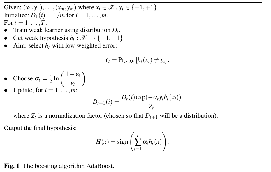
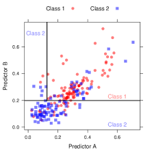
    1. It can become tricky as in case of XOR
    2. XOR is very famous case in classification literature 
  3. Stop if very few point are left in the node
    1. This works pretty well in practice
    2. Stop if node has say 10 to 100 sample

Pruning

  • Pruning generally is better solution than early stopping
  • Here we build the entire tree first and than remove certain node
  • Criterion for removing nodes:
    • cost(tree) = error(tree) + λ*L(tree)
    • L(tree) = no of leaf nodes
  • if cost(deep_tree) > cost(small_tree) then don’t split that node
  • Algorithm:
    • Start from bottom up the tree and traverse up and test one node each time
    • Calculate cost
    • Make decision to prune it or not

References:

Course by University of Washington

https://www.coursera.org/learn/ml-classification

Handling missing values in Decision Tree

We had previously written about classification trees and regression trees.

In this blog we will mainly write about handling missing values specifically for decision trees.

Handling over-fitting for decision tree is described here.

Missing Values

Missing value can cause issues at :

  1. Training time
  2. Prediction time
    1. What if while prediction sample does not have value for some feature

Purification by Skipping

  • This approach involves skipping rows or entire features that contain missing values.
  • However, this method comes with a drawback as it results in the loss of valuable information.
  • It is important to note that skipping missing values during training will not resolve the issue during prediction time

Imputation

  • Imputation refers to the process of filling in missing values with estimated or imputed values.
  • It provides a means to address missing values during both training and prediction.
  • A dictionary can be created to store imputed values for each feature, which can then be utilized during prediction.
  • For categorical features, a common imputation method is to use the mode, while for numeric features, the average or median is often employed.
  • Advanced techniques, such as the expectation maximization algorithm, can also be utilized for imputation.

However, it’s essential to be aware that imputation can introduce systematic biases into the data. For example, let’s consider a scenario where people from Washington tend to not provide their age, while the rest of the United States does. This could lead to a systematic bias in the imputed values, as the imputation process may assign ages based on data from other regions.

Algo specific technique

In decision tree algorithms, there are specific techniques to handle missing values. At each node in the decision tree, we need to determine which branch the missing value will take. It’s possible for the same feature to have different values at different nodes. To address this, we can make a tweak in the decision tree algorithm:

  1. During feature selection, consider assigning the missing value to each possible branch.
  2. Evaluate the effect of assigning the missing value to each branch by measuring the reduction in classification error.
  3. Choose the feature and branch that result in the highest reduction in classification error when the missing value is assigned.

However, what if we encounter a node during prediction where we didn’t have any missing values during training? In such cases, we can store the direction with the most number of samples at that node as the default direction for missing values. Let’s call this direction “max_sample.”

If we encounter missing values while training the decision tree, we can override the default “max_sample” direction with the observed direction for the missing values.

By incorporating these techniques, we can effectively handle missing values in decision trees and make informed decisions based on the available data.

References:

Course by University of Washington

https://www.coursera.org/learn/ml-classification

AdaBoost

  • AdaBoost stands for adaptive boosting
  • Boosting is a technique for creating better classifier form several regular/weak/base classifiers
  • Thought:
    • We want to train second classifier in such a way that training data has more samples for the case where first classifier was wrong
    • Third classifier will have more samples where first and second classifier contradicts
  • How do we accomplish above:
    • We assign weights to each sample
      • This weights will be used in error function for each sample
      • Error function would be sum of weights of incorrectly classified samples
      • This weights keep changing in each iteration
    • We also assign wight to each base (weak) classifier (α In below algorithm)
      • Formula for calculating α below is valid for binary classification
        • It will be different for multi class classification
  • When do we stop iteration ?
    • Combined classifier is predicting all sample correctly
    • No more base classifier left
  • Most machine learning algorithms allows to apply weight to data
    • In logistic regression we can multiply weight in error fucntion
    • In decision tree, classification error can be calculated by summing weights of missclassified samples


adboost


Formulations in above algorithm:

  • Formula of α
    • if ε=0.5 then α=0. It is just a random chance classifier.
    • Else it can positive/negative.
    • ε < 0.5 => negative α => we invert the prediction in weighted average
  • Formula of D_(t+1)(i)
    • y*h is just a sign
      • y and h are  {-1, 1}
      • y*h will be positive for correct prediction
    • Why it is function of ε
      • Random classifier updating weights does not make sense
  • By Z_t we are normalizing weights, which ensures numerical stability


Adaboost Theorem

  • Error -> 0 as no of iteration -> infinity at certain condition
  • Condition is here is that each learner has error < 0.5
  • Each iteration means adding one weak learner


Over-fitting

  • Contrary to weak classifier (decision stumps) we saw that rate of increase test error is less with boosting
  • However no of iteration still should be selected via cross validation for small data-set and validation for large data-set


References:

Click to access MIT6_034F10_boosting.pdf

Click to access msri.pdf


Classification Trees

How classification Tree creates Rectangle in Predictor Space

Criterion for Choosing the Splitting Predictor

When deciding which predictor to split on, we need to consider different types of predictors: continuous, binary, and categorical. In this post, we will focus on continuous and binary predictors.

For categorical predictors, one approach is to use the “one vs rest” strategy. We evaluate each category separately and observe which one reduces the randomness the most when split.

In the case of a continuous predictor, we first sort the values and then select the midpoint as the split point.

To keep our decision tree simple, it’s ideal to have a small tree size. Therefore, at each step, we should choose the split that leads to the purest child nodes.

Two commonly used criteria for measuring impurity are Gini and Entropy. It’s important to note that these criteria are not directly used to select the predictor to split on. Instead, we calculate the difference in impurity before and after splitting.

When computing Gini or entropy after splitting, we apply weights to both splits to account for their proportions.

Multi-class

Decision tree can naturally handle multi class problem as entropy and gini can be calculated for multi-class.

Entropy

  • Formula:
    • H = ∑ -p * log(p)
  • About :
    • Randomness
    • Information Carries
    • Highest when p=0.5
    • Higher Entropy => Higher Randomness => Carries more information
    • After splitting we want entropy to reduce
  • Initial :
    • n0 positive and m0 negative sample
    • g0 = (n+m) total samples
  • After Splitting
    • Group 1:
      • n1 positive
      • m1 negative
      • g1 = (n1 + m1) total
    • Group 2:
      • n2 positive
      • m2 negative
      • g2 = (n2 + m2) total
  • Before Entropy :
    • H_before =  -(n0/g0) log(n0/g0) – (m0/g0)log(m0/g0)
  • After Entropy :
    • H1 = -(n1/g1) log(n1/g1) – (m1/g1)log(m1/g1)
    • H2 = -(n2/g2) log(n2/g2) – (m2/g2)log(m2/g2)
    • H_after = (g1/g0) * H1 + (g2/g0)*H2
  • diff = H_before – H_after
  • Select a predictor for which diff is highest and split on it
    • Which means we are selecting a predictor which reduces randomness more
    • Which also mean we are selecting a predictor which reduces information more
      • So we are selecting a variable which carries more information
        • More important feature

Gini

  • Gini for 2 class :
    • G = p1 * (1-p1) + p2 * (1 – p2)
    • Using (p1 + p2 = 1) we can derive that G = 2*p1*p2
  • Gini in general:
    • G = ∑ p * (1 – p) = 1 – ∑ p²
  • Like entropy gini is maximum when p1 = p2 = 0.5
    • In this case nodes are least pure
  • Gini is a measure of impurity which we want to reduce by splitting on predictor
  • diff = G_before – G_after
    • We will select a predictor for which diff is highest

Entropy vs Gini

  • Given a choice gini will be better as computing log is costlier.
  • Both of them are better than “classification error as metric” [1]
    • Which would be selecting majority class for calculating classification error
    • It is useful while pruning but not while growing the tree

ROC Curve

  • ROC curve can be constructed easily for classifier which outputs ranking.
  • On the contrary decision tree outputs label
  • However to get a ROC we can use workaround. Each leaf node will have some positive and negative samples and we can calculate probability as (# positive / # total).
  • Then we can change the threshold and plot ROC.

Regularization

Regularization in decision tree will be explained in separate blog in detail, but here is the list of candidate techniques.

  1. limit max. depth of trees
  2. Cost complexity pruning
  3. ensembles / bag more than just 1 tree
  4. set stricter stopping criterion on when to split a node further (e.g. min gain, number of samples etc.)

Reference

[0] : Applied predictive modeling by Max Kuhn and Kjell Johnson

[1] : https://github.com/rasbt/python-machine-learning-book/blob/master/faq/decision-tree-binary.md