Anomaly Detection Basics

These are notes form Andrew N.G’s machine learning course on coursera.

Anomaly Detection Problem

  • Assembly line prepared aircraft engine, you want to check if it okay.
    • Features can be
      • heat generated
      • vibration intensity
  • Fraud detection in finance/retail
    • Feature would be based on user’s activity
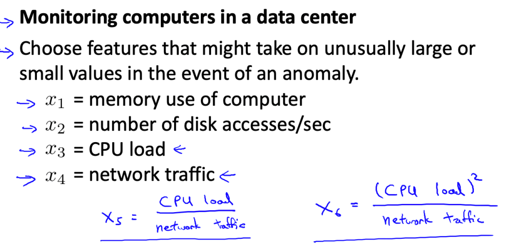
  • Monitoring CPUs in data center
    • Features would be memory used, CPU load, network traffic.
  • Generally we have less number of positive (anomalous example) compared to negative ones (normal).

Solution Based on density Estimation

  • We try to fit normal examples in gaussian distribution
  • For new engine we estimate the probability of it p
  • If p < epsilon – we flag the new engine as anomalous
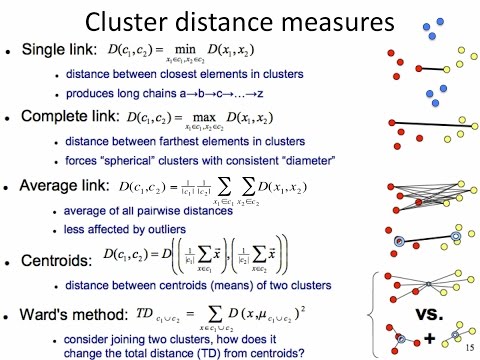
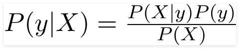
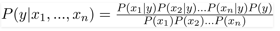
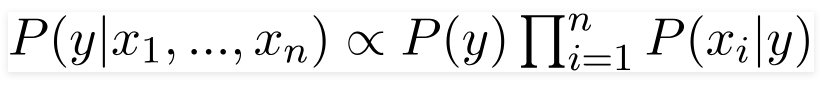
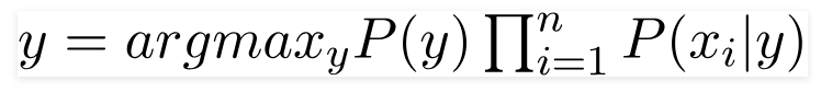
  • We generally train one gaussian per features and multiply like naiver bayes
    • That is to say off diagonal elements in multivariate gaussian are zero
    • More details in the last section of this post ( multivariate gaussian )

Model Evaluation

  • Once we have multiple models having different features how to evaluate which one is better ?
  • We also need to tune epsilon parameter.
  • We can use standard setup of train-set, test-set and cross validation set
  • Train set would have normal examples only. It would okay if few anomalous samples slips in
    • So training is unsupervised only
    • Predict y = 1 if p(x) < epsilon else 0
  • Bad metric
    • classification accuracy (because classes are imbalanced)
  • Good metric
    • TP, FP, TN, FN
    • Precision/recall
    • F1 score
  • Cross validation set is used for tuning epsilon

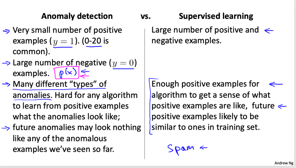
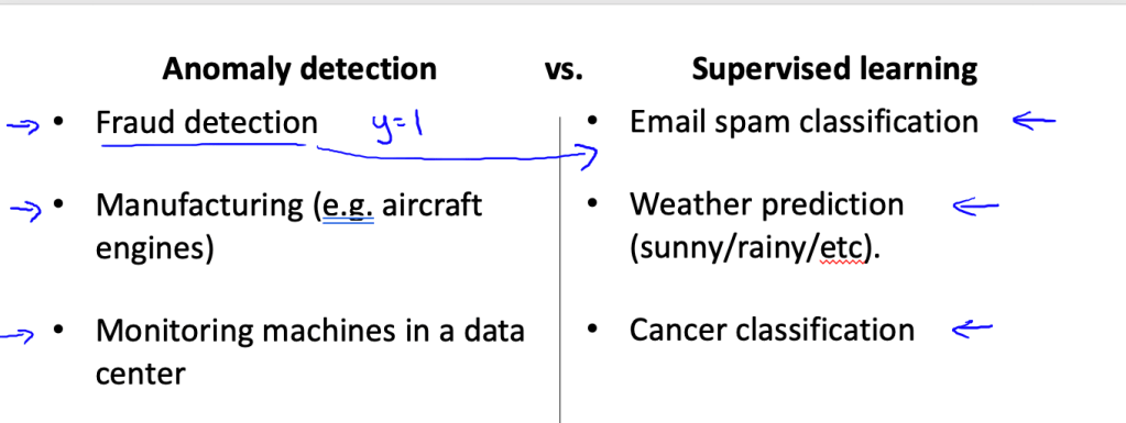
Anomaly Detection vs Supervised Learning

  • Supervised model like logistic regression would require
    • 1) More training examples
    • 2) Somewhat balanced classes

Feature Engineering

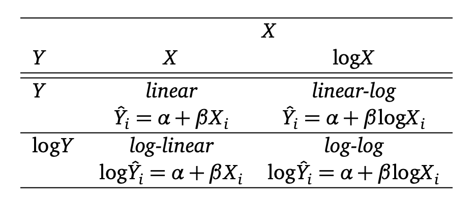
  • Since we are fitting gaussian we need to do some transformation if feature distribution does not look like one. Popular transformations are
    • log (x)
    • log (x + c)
    • sqrt (x)
  • How to introduce new feature
    • We need to do this when p(x) is comparable for normal and anomalous sample
    • Once you find anomalous sample for which p(x) is not low enough, try looking deep into it.
    • Property which is making it anomalous would be a new feature to add
  • Feature Engineering Recommendation
    • Think about features which will be too high or too low in case of anomaly
    • x5 and x6 can be a good feature in below image.

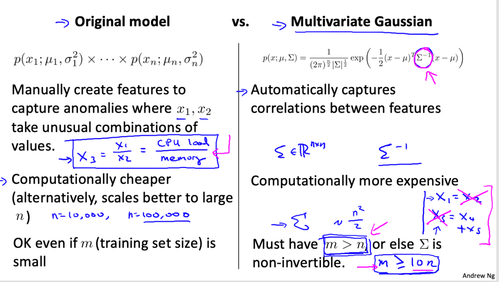
Multivariate Gaussian

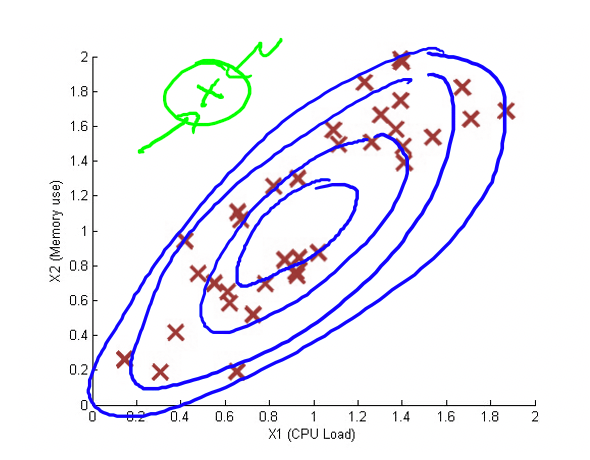
  • Shortcoming of individual gaussian is that in case of correlated features it won’t be able to detect the anomaly.
    • Green sample in above image will not be detected
  • To mitigate this we can hand-code ratio based features
  • Original model is more popular because it scales well with no of features.

Gradient Boosting

Some people use term bagging and boosting, some use parallel and sequential ensembles. I have written a post on AdaBoost previously. So we are familiar with boosting idea.

In AdaBoost we had a formula for generating labels (label/sample weight in loss function to be precise) for next iteration. In gradient boosting we fit gradient of loss function with respect to predictions.

Prof Balaraman notes

  • Most of this post contains info from [0]. However Prof. Balaraman offers intuitive perspective in one of his lectures. [3]
  • My handwritten note on that is available at [2]
  • We can write decision tree as equation where regions and value in the region are parameters.
  • Two steps of gradient boosting
    1. Fit gradient of loss function using regression trees (least square loss)
    2. Compute values in region using loss defined for application (ndcg for ranking, log-loss for classifier anything)
  • Whatever is application loss, we fit regression tree using least square
  • Parametric gradient descent can be seen as series of summation starting from initial guess.
  • Related paper [4]

Basis Functions

  • Basis functions
    • If we want to fit non linear curve with simple linear regression, we will create polynomial features
    • It is not limited to regression though
  • Adaptive Basis function
    • Instead of we defining above functions, we learn them
    • This can be framed as optimisation problem and can be solved by gradient descent/newton’s method for some hypothesis space
  • How to include Tree’s in base hypothesis space
    • Something which we can not differentiate
    • Even if we fix parameters to split on output is still not continuous
    • So it is difficult

FSAM

  • FSAM
    • Forward Stage-wise Additive Modelling
    • AdaBoost is example of this, another example is L2 boosting
    • We can say weak function is step direction and coefficient is step size
  • L2 Boosting also example of FSAM
    • We are fitting residual
    • To prevent overfitting we can reduce step size
    • If v*h(x) is also in H, we can remove v. (closed under rescaling)
    • h(x) can be decision stump we can keep going as long as residuals exist (It will certainly overfit after few iterations)
  • Adaboost
    • It works for classification problem
    • When the loss function in FSAM is exponential loss of margin, it reduces adaboost
    • margin = y*f(x)
      • We had encountered that in SVM
  • Disadvantages of AdaBoost
    • Gives too much penalty for negative margin, look at the curve of exponential above
    • Mislabel training data
    • Sometimes there is noise in world
    • Does not work when there is high baye’s error
    • Also it seems AdaBoost formulation is very much tied to classification
      • We probably needs to tweak it to apply it to ranking problem
      • But gradient boosting can be applied to any problem (loss function)
        • Because Tree is alway using L2 loss
Slide from [1]

Functional Gradient Descent

  • Gradient is pseudo residuals
    • For L2 loss it is actually residuals (difference between y and f)
    • Examples where residuals are not just difference between y and f
      • logistic loss
      • ranking using ndcg
  • We fit this gradient(pseudo-residuals) with weak function
    • Regression Tree is most common
    • We find closest approximation to gradient step in base hypothesis space (which is functional space)
    • Here we minimize square loss (regression problem)
  • Earlier tree used to be just stumps
    • That is num of leaf node = 2
    • Now a days xgboost/light gbm takes upto 8/16 leaf nodes as well
  • Note that while calculating gradient the hypothesis function is not involved anywhere
  • How do we calculate gradient over function space
    • In close form expression it might look complicated
    • From numerical computation perspective we need gradient at just one point (of dimension training data size)
    • This is just like taking gradient of weights in linear regression
      • Here size of gradient vector would be number of training examples
    • In most of the method we take gradient of parameters, here we are taking gradient of predictions
  • What should be step size
    • Line search
    • Regularisation parameter (similar to what we use for any gradient based optimisation)
      • This is more common

Reference

[0] https://www.youtube.com/watch?v=fz1H03ZKvLM

[1] https://davidrosenberg.github.io/mlcourse/Archive/2016/Lectures/8b.gradient-boosting.pdf

[2] https://github.com/arcarchit/datastories/blob/master/notes/gradient_boost_iitm.pdf

[3] https://www.youtube.com/watch?v=FJ-MA0EfJ9k

[4] https://statweb.stanford.edu/~jhf/ftp/trebst.pdf

log-linear and log-log regression

In linear regression taking log is popular way to make relationship linear. We can take log of either response or predictor or both. This gives us four classes [0]

log_llog

Interpretations of β

  • Linear Model
    • the coefficient β gives us directly the change in Y for a one-unit change in X
  • Linear Log Model
    • β is the expected change in Y when X is multiplied by e (natural log)
  • Log Linear Model
    • Each 1-unit increase in X multiplies the expected value of Y by e β
  • Log Log Model
    • multiplying X by e will multiply expected value of Y by e βˆ

I have coded notebook to see the curves for all four at [1]. 

A note on Normalisation

  • Suppose you need to normalise a data to bring it between 0 and 1. This will be feed into some linear function (say ranking function without supervised response y). If you data is exponentially distributed instead of dividing by max, you can try log(sample)/log(max).  This is like feature transformation by taking log and then normalising it.
    • That’s about normalising variable which seems to have exponential distribution
  • Also when you check correlation with response variable and you see plots like [1] you know which transformation to take.
References :

[0] https://kenbenoit.net/assets/courses/ME104/logmodels2.pdf
[1] https://github.com/arcarchit/datastories/blob/master/notebooks/log_linear_models.ipynb

Clustering Metrics

Here are some metric available for validating clustering, explanation of each one is available on sklearn. [0]

If ground truth labels are available:

  • Adjusted Rand Index
  • Mutual Information Based scores
  • Homogeneity, completeness and V-measure
  • Fowlkes-Mallows scores

If not available :

  • Silhouette Coefficient
    • Range (-1,1)
    • 1 means it is similar to data-points in each cluster
  • Calinski-Harabaz Index
  • Davies-Bouldin Index
  • Contingency Matrix


Calculating SSE

It is a sum of distance between each point and its cluster center.

c1

Silhouette Score

It is calculated for each point and then we take an average of it.

c2

c4           c3

a(i) is average distance of a point to other points in same cluster.

b(i) is minimum of above average in for point in other cluster. It given the distance to nearest cluster.

s(i) close to 1 means data point is appropriately clustered. -1 means it is very bad clustered.

Setting s(i) to 0 when cluster size is one ensures that curve is not monotonically decreasing.


Elbow method and Silhouette Analysis

Notebook is available at https://github.com/arcarchit/datastories/blob/master/Silhouette.ipynb

sil1         sil2

Rand Index

  • When cluster labels are available we can use this matrix
  • It basically checks the similarity between two cluster assignments
    • Labels can also be seen as one type of cluster assignment
    • Score basically tells us how similar to cluster assignments are
  • This works by taking pair of points
    • Out of all pairs how many pairs are agreed in both clusters mechanism
    • Agree mean both
      • They are in same cluster in both mechanism
      • They are in different cluster in both mechanism
  • The Rand index has a value between 0 and 1, with 0 indicating that the two data clustering do not agree on any pair of points and 1 indicating that the data clustering are exactly the same

rand_index

  • One drawback of Rand index is that it can given non zero value for random assignment of clusters. To mitigate that there is matrix called Adjusted Rand Index. [2]
    • It specifically does not work when no of clusters are high


Reference

[0] : https://scikit-learn.org/stable/modules/clustering.html

[1] : https://github.com/anthonyng2/udemy-the-complete-machine-learning-course-with-python

[2] : https://davetang.org/muse/2017/09/21/adjusted-rand-index/


Oversampling and Under-sampling

When data is class-imbalanced there is a tendency to predict majority class. One way to tackle this would be apply more weight to minority classes in cost function. Another way is oversampling and under-smapling.

  • Over-sampling makes duplicate copies of minority classes
  • Under sampling randomly removes some samples from majority class
    • This should be used with caution
    • We need to check once that we still remain with enough sample for a given no of features
  • Practically we might want to over sample some classes and under-sample others.


Cross validation

  • Validation set should be taken out from original data[1]
    • We can do the sampling just before training only on training data


Reference

[0] : https://www.kaggle.com/residentmario/undersampling-and-oversampling-imbalanced-data

[1] : https://www.marcoaltini.com/blog/dealing-with-imbalanced-data-undersampling-oversampling-and-proper-cross-validation


Generative and Discriminative Models

Introduction

In machine learning, there are two broad categories of models: generative models and discriminative models. In this blog post, we will discuss some popular examples of each and their capabilities.

Generative Models

  1. Naive Bayes Classifier
  2. Hidden Markov Models
  3. Latent Dirichlet Allocation
  4. Boltzmann Machine
  5. Gaussian Mixture Model ( Unsupervised clustering)

Generative Models Explanation

Generative models allow us to generate datasets for specific classes, labels, or clusters. They estimate the joint probability distribution P(X, y). An example of this is the Naive Bayes Classifier, where we have a probability associated with each (X, y) pair. For classification, we predict y based on the highest probability given x.

𝑎𝑟𝑔𝑚𝑎𝑥𝑦𝑃(𝑌=𝑦|𝑋=𝑥)=
𝑎𝑟𝑔𝑚𝑎𝑥𝑦𝑃(𝑌=𝑦,𝑋=𝑥)/𝑃(𝑋=𝑥) = 𝑎𝑟𝑔𝑚𝑎𝑥𝑦𝑃(𝑌=𝑦,𝑋=𝑥)/𝑃(𝑋=𝑥)

Generative models offer more than just prediction. They can be used to:

  • Impute missing data
  • Compress datasets
  • Generate unseen data

Discriminative Models

  1. Logistic Regression
  2. Support Vector Machines
  3. Decision Trees

Discriminative Models Explanation

Discriminative models focus on learning the boundaries that separate different classes directly. They do not model the entire joint probability distribution but instead estimate the conditional probability P(y|x). Examples of discriminative models include Logistic Regression, Support Vector Machines, and Decision Trees.

Hidden Markov Models

From a Clustering Perspective

This section summarizes a lecture from the University of Washington [0] on clustering time series data, considering the significance of both the data and indices.

Other potential applications include:

  1. Honey bee dance: Bees switch from one dance to another to convey messages.
  2. Conference conversations: Segmenting speaker assignments based on the spoken turns.
  3. Gym exercises: Identifying exercises from pulse rate data as people switch between activities.

Model

The following screenshots are from a YouTube video [1] by the Mathematical Monk, illustrating the model:

Suppose you’re developing handwriting recognition and need to recognize a hidden variable.

The prediction for “i” depends solely on the previous character being “h,” disregarding how “h” was written.

hmm_concept
hmm_parameters

Code and Notebook

You can find the code and notebook at the following GitHub link [2], which extensively explains:

  1. The structure of the model.
  2. The forward algorithm for calculating the likelihood of a given observation.
  3. The backward algorithm for finding the most probable state sequence given an observation (also known as decoding).
  4. The forward-backward algorithm for inferring model parameters from a set of observed sequences.

References

[0] : https://www.coursera.org/learn/ml-clustering-and-retrieval/home/welcome

[1] : https://www.youtube.com/watch?v=TPRoLreU9lA

[2] : https://github.com/arcarchit/datastories/blob/master/hmm.ipynb

[3] : https://web.stanford.edu/~jurafsky/slp3/A.pdf

Hierarchical Clustering

This post is a lecture summary of  course by University of Washington : https://www.coursera.org/learn/ml-clustering-and-retrieval/home/welcome


Why one might want to use hierarchical clustering ?

  • A common problem is clustering is to predefined no of clusters (k)
    • Hierarchical clustering does not need that
  • Deprogram provides effective visualization of clusters at various levels without re-running the algorithm
  • Any distance metric can work, while k-mean required euclidean distance [0][1]
  • We can construct more complex shape compared to k-means/EM


Divisive clustering

  • Example algorithm is recursive k-mean
  • We first cluster with k = 2 and then recursive apply k-means on these two clustersdivisive_clustering
  • Various choices we need to make :
    • Which algorithm to use (k-means)
    • How many split at each level (k=2, 3)
    • When to stop? Here are some heuristics:
      • Number of points in a cluster falls below certain threshold (Minimum point in each cluster)
      • Distance to farthest point falls below certain threshold (Minimum cluster radius)
      • Until per-specified no of clusters are reached


Agglomerative clustering

  • Example would single linkage algorithm
  • We start with assigning each point to its own cluster
  • Next task is how to merge this cluster
    • How do we define the distance between cluster?
      • Linkage function
        • It gives us two points from each cluster
        • Single linkage given points which has minimum distance across all possible pairs
        • Cluster A has points (a1, a2, a3) and B has (b1, b2, b3)
        • Linkage will give say (a2, b3) if it has the minimum distance across all combination
      • Distance Function
        • Can be euclidean or cosine anything
    • We merge the cluster which has minimum distance
  • Dendrogram provides efficient visualization [4]
    • Data-points of x-axis carefully ordered
    • Height (y-axis) represents distance between two cluster as per specified linkage
    • It gives us the complete visualization of which nodes were merged first followed by which one etc.
  • How to cut dendrogram ? [4]
    • Suppose we are cutting the dendrogram at y=D*
    • There are no pair of cluster which has distance < D* and which is not merged
    • All the pairs of clusters having distance < D* are merged
    • D* is the minimum distance between cluster at this level
    • Distance between clusters identified > D*
  • Various linkage functions [2][3]
    • Complete linkage takes two farthest points
    • Average linkage considers all pairs and takes an average
    • Ward linkage focus on increasing sum of squares
    • These linkage however brings down the shaping flexibility
      • Single linage would allow for complex shapes in general
      • Single linkage however can result in chaining
  • Choice we need to make in agglomerative clustering
    • Which linkage function to use
    • Which distance metric to use
    • Should we cut dendrogram flat or some weird cut

dendrogram

  • Complexity
    • For brute-force it is O(N^2 log N)
    • We can also prune search space by kd-trees or using triangular inequality
    • Best know is O(N^2) [5]


Linkage Functions

linkage

References

[0]: https://stats.stackexchange.com/questions/81481/why-does-k-means-clustering-algorithm-use-only-euclidean-distance-metric

[1]: https://pdfs.semanticscholar.org/a630/316f9c98839098747007753a9bb6d05f752e.pdf

[2] : https://www.saedsayad.com/clustering_hierarchical.htm

[3] : https://stats.stackexchange.com/questions/195446/choosing-the-right-linkage-method-for-hierarchical-clustering

[4] : http://www.econ.upf.edu/~michael/stanford/maeb7.pdf

[5] : https://www.cs.ucsb.edu/~veronika/MAE/summary_SLINK_Sibson72.pdf

Which ML algorithm to use when?

We generally find this question while starting up new project or we want to compare some algorithms to discriminate them (discrimination helps understand things better sometimes).

Although there is no definitive answer to this, I am writing here summaries from some posts. [0]


machine-learning-cheet-sheet


Factors to consider

  • Accuracy
    • Most of people focus on accuracy but it practically it is not the only
  • Training time
    • Naive Bayes and logistic regression are much faster than boosting or neural nets
  • Linearity
    • LR and SVM are suitable when classes are linearly seperatble
      • Of course SVM bypasses it via kernel trick but still not as much complex decision boundary as nueral nets
    • Despite the risk of non linearity in data linear algorithms tends to work well in practice and are often used as starting point
  • Number of parameters
    • Parameters does affect training time and accuracy
    • More parameters helps learning complex function, however it requires more data to prevent over-fitting
  • No of features
    • When data point are not enough for no of features (text, NLP) SVM works well


Notes

  • Try out linear/logistic regression, SVM first when you most dependent variables are numeric.
  • SVM
    • SVM suites more when no of data points are less for given no of features.
    • SVM is linear classifier only. It just uses kernel trick to project linearly inseparable data on high dimension.
    • SVM is solved by mathematical optimization problem unlike nueral nets. Hence tends to be bit faster.
  • What is the difference between LR and SVM?
    • LR has linear decision boundary while SVM can have non linear decision boundary.
  • Reinforcement learning
    • Analyses and optimized behavior of agent, (via feedback from environment)
    • They try to discover different actions to maximize reward
    • Trial-error and delayed reward distinguishes reinforcement learning from other ML algorithms


References

[0] : https://blogs.sas.com/content/subconsciousmusings/2017/04/12/machine-learning-algorithm-use/#prettyPhoto

[1] : https://docs.microsoft.com/en-us/azure/machine-learning/studio/algorithm-choice


Naive Bayes Classifier

  • There are two things[1]
    • Probability model
    • Classification model

Probability Model

A probability model is an extension of Bayes’ rule. It makes two assumptions:

  1. Independence of Features: This assumption assumes that all features are independent of each other. However, it does not hold true in many cases. For example, having higher temperature does not necessarily imply higher humidity.
  2. Equal Weight of Features: This assumption assumes that all features have equal importance or weight in the model.
b1
b2

Classification Model

The classification model involves the following steps:

  1. Probability of Each Class: P(y) represents the probability of each class based on the training set.
  2. Probability Estimation of Feature Values: The goal is to estimate the probability distribution of each feature value given a specific class, denoted as P(x_i|y). For discrete features, this can be achieved through simple probability calculations, such as multinomial Naive Bayes. For continuous features, Gaussian distributions can be used. In the case of count data, multinomial distributions are suitable.
  3. Parameter Estimation: Parameter estimation is performed for each combination of class and feature.
  4. Scikit-learn and Distribution Types: Scikit-learn library provides implementations of Gaussian Naive Bayes, Bernoulli Naive Bayes, and multinomial Naive Bayes classifiers. These classifiers refer to the distribution of features. It is important to note that different features can follow different distributions. Therefore, customization of the distribution based on the application may be necessary.
b3
b4

Advantages

  • Fast and Easy Implementation: Naive Bayes classifiers are known for their simplicity and efficiency in implementation.
  • Acceptable Classification Performance: While Naive Bayes classifiers may not always accurately predict probabilities, their classification performance is generally satisfactory.

Disadvantage

  • Independence Assumption: The assumption of feature independence does not hold true in all scenarios, which can affect the model’s accuracy.

Reference

[0] https://towardsdatascience.com/naive-bayes-classifier-81d512f50a7c

[1] https://en.wikipedia.org/wiki/Naive_Bayes_classifier