Moving average and Auto-regressive Processes

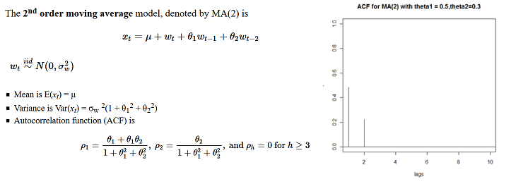
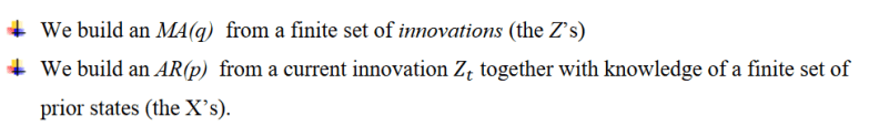
Moving Average Processes MA(q)

  • Stock price depends on announcements of last two days
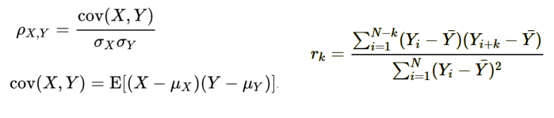
  • Auto correlation function cuts off at q

maq


Auto regressive Processes AR(p)


1

2

3


  • Below are the plots for AR(2) process
  • Depending upon the value of phi1 and phi2 ACF has alternative positive and negative values


56


Writing AR(p) process as MA process by substituting values of X(t-1). And yes phi is constant, we don’t need phi1, phi2 anymore.

78


Mean, variance and auto-correlation of AR(p) process, we have assumed Z = Norm(0, sigma2)

9


ACF of AR-p using Yule-Walker Equation

  • It is a method of solving difference equation in recursive relation
  • We first obtained auxiliary equation (also known as characteristic equation) which is polynomial and find root of that
  • Using these root we get weighted geometric series and find weights using some initial condition
  • We had learned in mathematics that this way of solving difference equation also related to solving differential equations
  • In the course they had solved it for Fibonacci series and root had come out to be golden ratio
  • For AR(p) ACF comes out to be difference equation, solving which can give us ACF for different values of lag


Reference

https://www.coursera.org/learn/practical-time-series-analysis/home/welcome

https://en.wikipedia.org/wiki/Autoregressive%E2%80%93moving-average_model


[Time Series] Correlation and Stationarity

Co-variance vs Correlation

  • Correlation is co-variance divided by standard deviation of both variables
  • Hence it is independent of units and is always between -1 and 1, which makes comparison easier
  • Formula on the right is time series specific
    • It is auto correlation coefficient at lag k
    • It is define as ration of auto-correlation at lag k divide by auto-correlation at lag 0
    • This values are plotted on correlogram  (See one for MA(2) process below)

acf


Stationary Time Series

  • No systematic change in mean (No trend)
  • No systematic change in Variance
  • No periodic variation (Seasonality)

If time series is not stationary we apply several transformation to make it stationary.

For example applying difference operator to random walk makes it stationary.


Random Walk

  • Previous value of noise
  • If first value is zero then current value is summation of all the noises so far
  • X(t) = X(t-1) + Z(t)
  • Z(t) = Normal (mu, sigma2)
  • if X(0) = 0 then X(t) = sum(Z(k)) k form 0 to t
  • Expectation[X(t)] = t*mu   – –  Changes with time
  • Variance[X(t)] = t*sigma2   – – Changes with time
  • Not a stationary process
  • let Y(t) = X(t) – X(t-1) = Z(t)  – – Y(t) is a stationary process


Example of Stationary Process

Moving average and Auto regressive processes described here can be stationary under conditions described here.


References


Further reading