Recommendation System Fundamentals

This are summaries from Andrew N.G’s course on machine learning.

Problem formulation of recommendation system

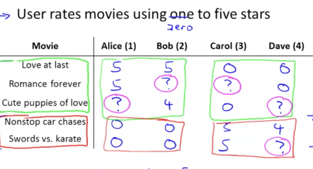
  • For this post we will use movie recommendation as example
  • We want to recommend movies to user
  • We will have ratings for some (user, movie) pair and would want to predict ratings for other pair
    • Then for a given user we will recommend movies sorted by highest prediction ratings
  • Two kinds of recommendation system
    • Content based
    • Collaborative filtering
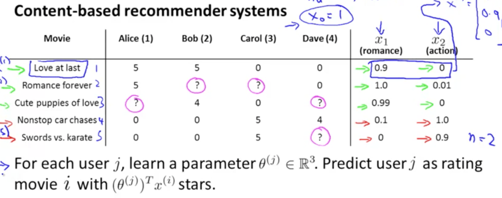
  • Content based recommendation
    • Each movie has some features
    • Train regression model for each user to predict ratings based on movie’s features

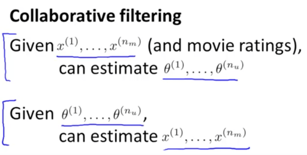
Collaborative Filtering

  • We need to know two things
    • Feature values for each movie
    • Weight parameter for each user
  • If we know one, we can calculate other
    • We will of-course consider (customer, movie) ratings
    • We have partially filled matrix as training set.
  • Can we do a joint optimisation for both ? That’s the idea behind collaborative filtering.
  • Why it is called collaborative filtering ?
    • Users are collaborating with each other to generate predictions for each other.

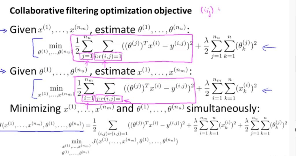
  • Notes of collaborative filtering equations
    • Both summations are equal.
    • x0 = 1 is not needed. x0 is constant term in linear regression
      • If model thinks it needs a feature which is constant it will create this on its own.

Collaborative filtering is essentially a matrix factorisation. We can construct matrix for movie and user based on vectors x and theta in above formulation.

  • Low rank matrix factorisation
    • Let number of user’s be nu
      • Number of movies nm
      • Number of movie feature k
    • User matrix dimension -> nu x k
      • For each user we have vector representing feature weights
    • Movie matrix dimension -> nm x k
      • For each movie we have feature value
    • Original matrix dimension -> nu x nm
    • We have factorised matrix into low rank k <= min(nu, nm)
    • It is very popular mathematical technique to discover latent structure with sparse data. [1]
  • Further application
    • Showing related item is different problem than recommendation
    • With collaborative filtering we are obtaining feature vectors for each movie/item
    • We can apply nearest neighbour on top of it

Cold start Problem

  • Mean normalisation helps combating that
  • In most ML algorithm we normalise feature (column)
  • Here you would like to normalise row from product perspective. Mathematically you can do both.
  • Example below
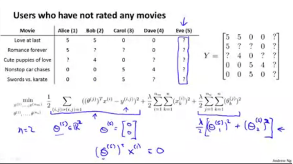
    • 5th user has not rated any movie (blue column in first matrix)
    • Regularised objective will make theta 0 for 5th user, which in turn produce 0 rating while making prediction
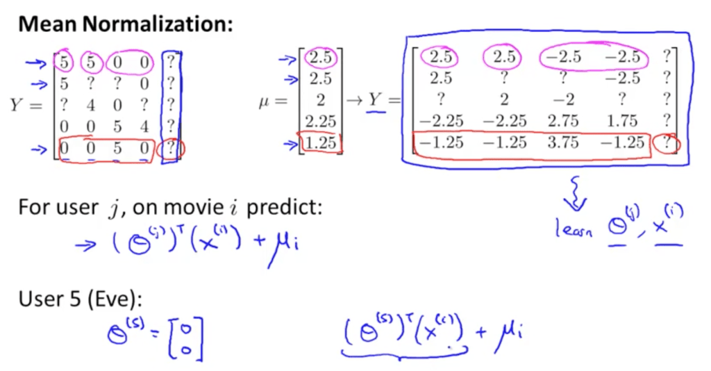
    • Mean normalisation transform Input matrix as shown below
    • During prediction time we add mean value for that movie
      • Theta will still be 0 for 5th user from matrix factorisation
      • After multiplying with 0 we are adding mean value to it

Reference

[1] https://arxiv.org/pdf/1507.00333.pdf

KL Divergence

We need to understand this four terms from information theory:

  1. Self Information
  2. Entropy
  3. KL Divergence
  4. Cross Entropy

Self Information

  • Information conveyed by any event
  • Higher the probability lower the information conveyedScreenshot 2019-11-24 at 4.38.31 PM

Entropy

  • Self information is of individual event, entropy is of distribution
  • Entropy is expected information of an event drown from that distribution
  • Distribution that are closer to uniform have highest entropy
    • Distribution that are nearly deterministic (where outcome is almost certain) have lower entropy
  • If log base is 2, it represents no of bites needed on average to encode symbols drawn from distribution of P. However this intuition is used prominently in communication theory than in machine learning.

Screenshot 2019-11-24 at 4.38.37 PM

KL Divergence

  • If we have two distribution P and Q of same random variable x, it tell how different this two distributions are

Screenshot 2019-11-24 at 4.38.43 PM

  • Extra amount of information (bits in base 2) needed to send a message containing symbols from P, while encoding was design for Q
  • KL divergence is always positive
    • It can be greater than 1
    • Bits required to encode information can be greater than 1
  • Example at [1]:
    • we have observed few events and we have the observed distribution
    • We want to represent is by some standard distribution say uniform or binomial.
    • Which one we should choose ?
      • The one for which KL divergence is minimum
      • This would same as to say the one for which extra information is minimum.
    • Binomial distribution has parameter p (probability of event = 1). Which value of this parameter we should choose ?
      • The one for which KL divergence is minimum.
      • It thus becomes an optimization problem
  • KL divergence is sometime termed as distance between two distribution
    • But it is not symmetric KL(P|Q) is not same as KL(Q|P)
  • Application :
    • One use case is in variational auto encoders (VAE) [2]
      • VAE generates sample data like GAN
      • For that we want output of encoder to be more generic before giving it to decoder
        • We measure this by measuring KL divergence of encoder output and uniform distribution
        • We add it in the final loss function

Cross Entropy

  • KL divergence measure extra information (bits) needed to encode P with symbols optimised for Q
  • Cross entropy measures total information needed to encode P with symbols optimised for Q
  • Formula for log-loss is exactly same (it is also called cross entropy loss)

Screenshot 2019-11-24 at 4.38.59 PM

Screenshot 2019-11-24 at 4.38.55 PM

Related

  • KS Test is used for goodness of fit
    • It is formulated in terms of hypothesis test and give p values
    • Based on empirical cumulative distribution function (empirical CDF)
  • KL divergence is differentiable
    • Popular in machine learning loss function
    • Based on information theory

References:

[0] : Deep Learning by Ian Goodfellow, http://www.deeplearningbook.org/

[1] : https://www.countbayesie.com/blog/2017/5/9/kullback-leibler-divergence-explained

[2]: https://towardsdatascience.com/intuitively-understanding-variational-autoencoders-1bfe67eb5daf