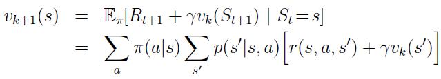
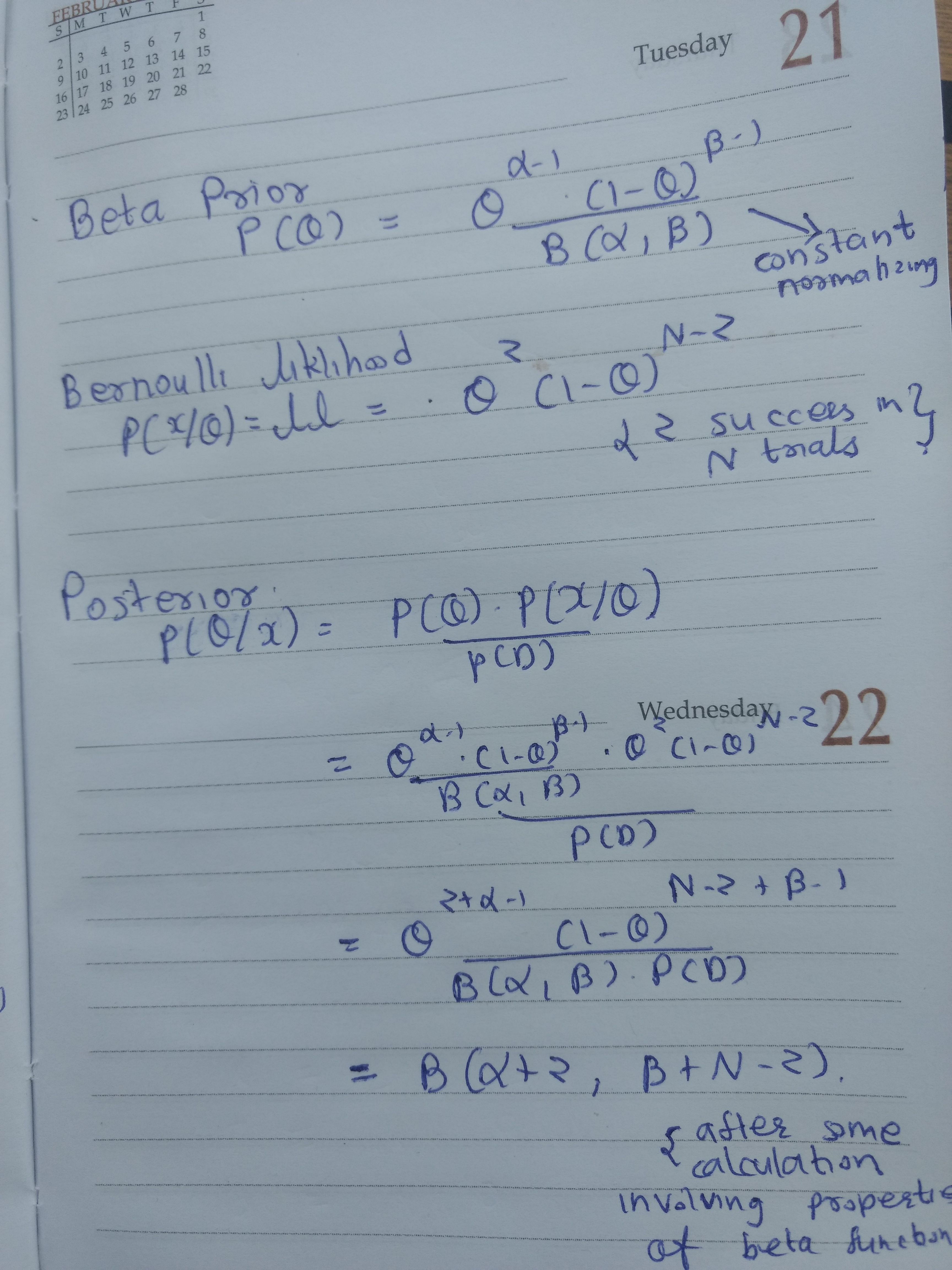
Q-Learning

Value Function

This represents value of a given state for the policy π.
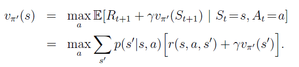
q1

Optimal Policy

q2

Learning Via Value Function is not possible when we don’t know immediate rewards and next state. If they are known we can use dynamic programming methods described at Dynamic Programming for RL.
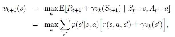
q3

Q function

q41

q42

How it solve the problem of unknown reward and next state functions?

  • To calculate value function we need to know immediate reward for next state and probability of moving into next state
  • In Q learning we are don’t need them
    • We just take best action, then observe the reward for whichever state we go in.
    • It is possible to know reward after taking action, not before that.


Training Rule for Q

We initialize Q table with random values and keep updating it on each action based on reward get.

q5

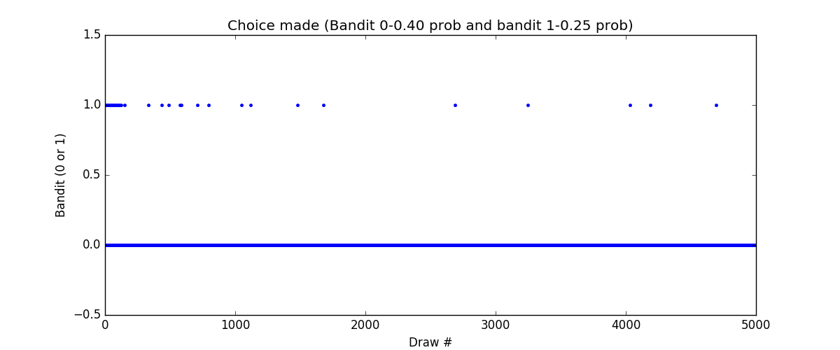
We have trained grid world with above equation. Notebook is available at [2]. One thing to note in that code is that, we don’t need backup. We don’t need to update entire q table simultaneously. We can calculate new value for once cell and write it at once.

Also [1] is a very good resource. It shows changes in the Q-update equation in non deterministic world. (Reward and next state are non deterministic).

qq3

And also derives TD updates (Temporal Difference)

qq4


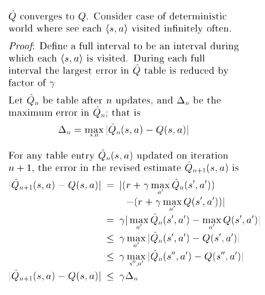
Convergence Conditions

  • System is deterministic MDP (Markov Decision Process)
  • Immediate reward values are bounded
  • Agent visit every state action pair infinitely often


Derivation for Convergence

q6

Experimental Strategies

  • We also need to do exploration
  • So we pick up action with a probability such that
    • action having more Q value has higher probability
  • One way to formulate this is as follows where in value of k control exploration-exploitation trade-off.
    • Initially k is small (exploration) and then is slowly increased (exploitation)

q7


How can we speed up Updating Sequence

  • Strategy 1
    • Consider the case for single absorbing goal state case. (What it means that if agent’s goal is to reach particular state) and initially all (q,a) pairs are initialized with 0.
    • So only one (q,a) pair will be update when we reach to reward state,
    • To speed up things, we can store intermediate state and action and then update backward till origin once we reach reward state.
    • Of course this will increase memory requirement
  • Strategy 2
    • Store immediate reward of past along with state-action pair and retrain periodically
    • If one Q(s, a) changes it will help change others as well
  • Strategy 3
    • If performing real environment action in environment is difficult we can perform simulation


Reference :

[0] Machine Learning by Tom Mitchell

[1] http://www.cs.cmu.edu/afs/cs.cmu.edu/project/theo-20/www/mlbook/ch13.pdf

[2] https://github.com/arcarchit/datastories/blob/master/RL_GridWorld.ipynb


Dynamic Programming for RL

Dynamic Programming is one of the method to solve reinforcement learning problem. It assumes that complete dynamics of MDP are known and we are interested in

  • Finding value function for given policy (Prediction problem)
  • Finding optimal policy for given MDP (Control problem)


There are three things :

  • Policy Evaluation
    • We calculate value of a given state
      • Average value given probability all actions defined in policy
    • Takes Probability of actions into account
  • Policy Iteration
    • First evaluates policy
    • Then generates new policy based on this evaluation
    • Calculates and updates maximum possible value of a state
      • Value is maximum when we take most optimal action
  • Value Iteration
    • Policy evaluation is time taking process
    • Let’s go with just one iteration
    • We don’t need to update policy in each iteration, just keep using new value function does the job
    • So it is like keep updating value function (choosing action that maximizes value instead of taking probabilities) until it converges and then selecting a policy based on this optimal values function
    • I have coded it at [0]


What is policy ?

A policy is simply a probability of performing an action (a) when in state (s) and our goal is to tune the policy to maximize the agents reward.


Different type of DP

Unlike traditional algo-ds problems this is a different type of dynamic programming. There mostly final ans is output of one cell, other cells are used for memoization. Here final answer is all the cells. We want to know value of all the cells. Another unusual DP problems are mentioned at [4].


Policy Evaluation

policy_eval

Policy Iteration

policy_iter

Values Iteration

value_iter


Here are two slides from : http://www0.cs.ucl.ac.uk/staff/d.silver/web/Teaching_files/DP.pdf


References

[0] : https://github.com/arcarchit/datastories/blob/master/RL_GridWorld.ipynb

[1] : Sutton’s book

[2] : https://github.com/dennybritz/reinforcement-learning/tree/master/DP/

[3] : http://www0.cs.ucl.ac.uk/staff/d.silver/web/Teaching_files/DP.pdf

[4] : https://github.com/arcarchit/mit-ds-algo/blob/master/dsalgo/cs/dp/dp_equations.md

OpenAI Gym Environment

Open AI provides framework for creating environment and training on that environment. In this post I am pasting a simple notebook for a quick look up on how to use this environments and what all functions are available on environment object.

I have used environment available on github by Denny Britz and here are the references :

References :

https://github.com/dennybritz/reinforcement-learning

Learning Reinforcement Learning (with Code, Exercises and Solutions)

https://gym.openai.com/docs/

My Code : https://gist.github.com/arcarchit/2b3363e2615df7ef5c8d4941d4dfa9e8


Loading

Sorry, something went wrong. Reload?
Sorry, we cannot display this file.
Sorry, this file is invalid so it cannot be displayed.

view raw

gym_env.ipynb

hosted with ❤ by GitHub

Thompson Sampling

Thompson sampling is one approach for Multi Armed Bandits problem and about the Exploration-Exploitation dilemma faced in reinforcement learning. It is also know as posterior sampling.

Challenge in solving such a problem is that we might end up fetching the same arm again and again. Bayesian approach helps us solving this dilemma by setting prior with somewhat high variance.

Here is the code for two armed bandit. One has success probability of 40% (bandit 0) and another has 25% (bandit 1).

We are using beta distribution for deciding which arm to pull. Beta distribution has two parameter alpha and beta. Higher values of alpha, pulls distribution towards 1. Beta distribution is always confined between 0 and 1.

How we train is that for each feedback we receive we increment alpha by 1 if it was success or beta by 1 in case of failure. For choosing the arm we draw random sample from the distribution of each arm and select the arm with highest value.

import numpy as np
import scipy.stats as stats
from matplotlib import pyplot as plt
class BetaThompson:
def __init__(self, num_bandits, prior_a, prior_b):
self.num_bandits = num_bandits
self.a = prior_a
self.b = prior_b
def learn(self, bandit, success):
if success:
self.a[bandit]+=1
else:
self.b[bandit]+=1
def suggest(self):
sampled_prob = []
for i in range(self.num_bandits):
dist = stats.beta(self.a[i], self.b[i])
prob=dist.rvs()
sampled_prob+=[prob]
return sampled_prob.index(max(sampled_prob))
class Gamble:
def __init__(self, num_bandits, binom_mean):
self.num_bandits=num_bandits
self.binom_mean=binom_mean
def gamble(self, bandit_no):
dist=stats.binom(n=1,p=self.binom_mean[bandit_no])
success = True if dist.rvs()>0.5 else False
return success
def main():
g = Gamble(2, [0.40, 0.25])
bot = BetaThompson(2, [1,1], [1,1])
choice=[]
for i in range(5000):
suggestion = bot.suggest()
result = g.gamble(suggestion)
bot.learn(suggestion, result)
choice+=[suggestion]
plt.figure(figsize=(12,5))
plt.plot(choice, 'b.')
plt.ylim([-0.5,1.5])
plt.title('Choice made (Bandit 0-0.40 prob and bandit 1-0.25 prob)')
plt.xlabel('Draw #')
plt.ylabel('Bandit (0 or 1)')
plt.savefig('choice.png')
if __name__== "__main__":
main()

And here is simulation results. We see that initially both the the armed are pulled frequently but slowly arm 1 is pulled less and less, but it is never straight away zero.

choice

Math Behind Increasing alpha and beta

In one line posterior is beta distribution for beta prior and Bernoulli likelihood. In other words beta is a conjugate prior for Bernoulli likelihood. List of various conjugate prior is available at [1].

PDF of beta distribution is simple once you think in terms of the effect of alpha and beta.

Look at note below, formula of beta distribution is not complex, actually it is very similar to

bayesian

References

[1] : https://ocw.mit.edu/courses/mathematics/18-05-introduction-to-probability-and-statistics-spring-2014/readings/MIT18_05S14_Reading15a.pdf