Microsoft had published a paper on RankNet in 2005, which also won ICML’s test of time award in 2015. Subsequent improvement to that algorithm were lambdaRank and lambdaMART. The later had also won 2010 – learning to rank challenge. Current paper[1] summaries all three algorithms and incremental improvement they are mapping. It is written by Chris Burges who was involved in these development since RankNet.
Quick Gist
- RankNet was trained using Neural Net.
- RankNet was trained to minimize pair-wise differences.
- LambdaNet was designed to maximise NDCG.
- Which is more relevant to IR compared to pair-wise differences.
- LambdaMART started using tree based boosting algorithms (MART, XgBoost etc)
RankNet
- For a given query (q), we have two items (i and j)
- I am writing down item but it would be any document (web page for example)
- We will have features for
- query
- item
- query item pairs
- For both (q, i) and (q, j) we pass them through NeuralNet and get scores -> si and sj
- We will also pass pairs which has same supervised label
- We need to decided a loss function based on si and sj, gradient of which we will back propagate.
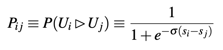
- Computed probability formula y_hat
- Supervised probability label y = (P_ij_bar) = (1 + S_ij) / 2
- S_ij = { 0, 1, -1}
- 1 if ( i is more relevant then j)
- 0 if (i is less relevant then j)
- 1/2 if both have same relevant scores
- y will be in {0, 1/2, 1}
- S_ij = { 0, 1, -1}
- sigma determines shape of sigmoid
- We would go to difference of (si – sj) on x-axis and read corresponding value from y axis.
- sigma determines steepness around 0
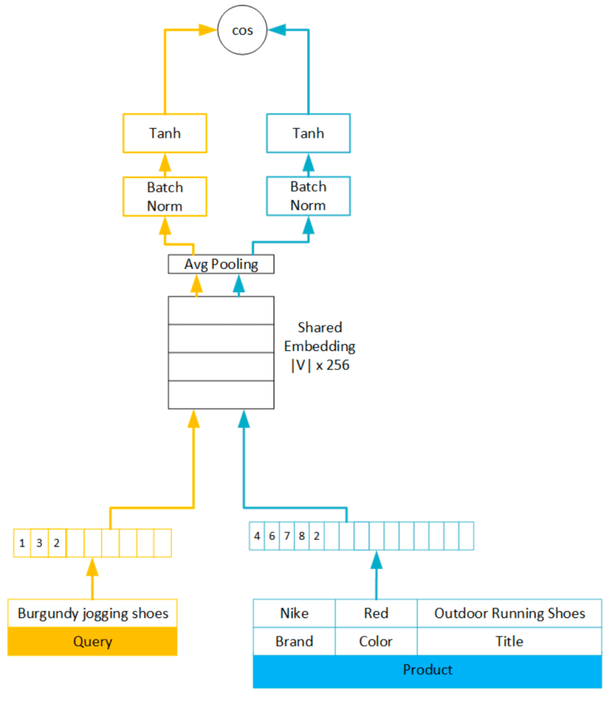
- This technique is known as temperature scaling. In tower network people use is when passing cosine similarity value to sigmoid.
- Technique is useful when input has limited range
- Cosine similarity has range (-1, 1)
- s_i – s_j would also have smaller range
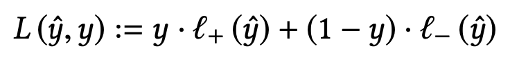
- Cost function is cross entropy
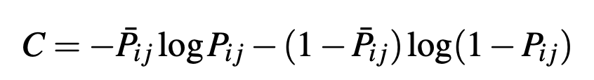
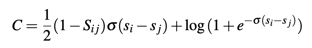
- One observation here is that when si = sj
- cost = log 2 > 0
- Document with different label but same score are still pushed aways from each other.
Speeding up RankNet Training by factoring
Defining lambda_ij
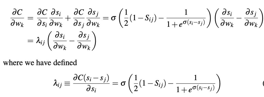
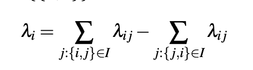
Defining lambda_i
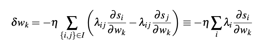
- What speedup did we achieve
- Earlier for a given query we were computing lambda_ij for each pair and updating weights
- Now we are computing lambda_i for each document and then update weight for given query
- You can correlate this to going from SGD to mini-batch
- We can do SGD at query, pair level or query level. We choose later.
- Intuition of lambda_i
- Direction(+Ve/-Ve) and magnitude where we want document to move
- Move up/down in the ranking
- Direction(+Ve/-Ve) and magnitude where we want document to move
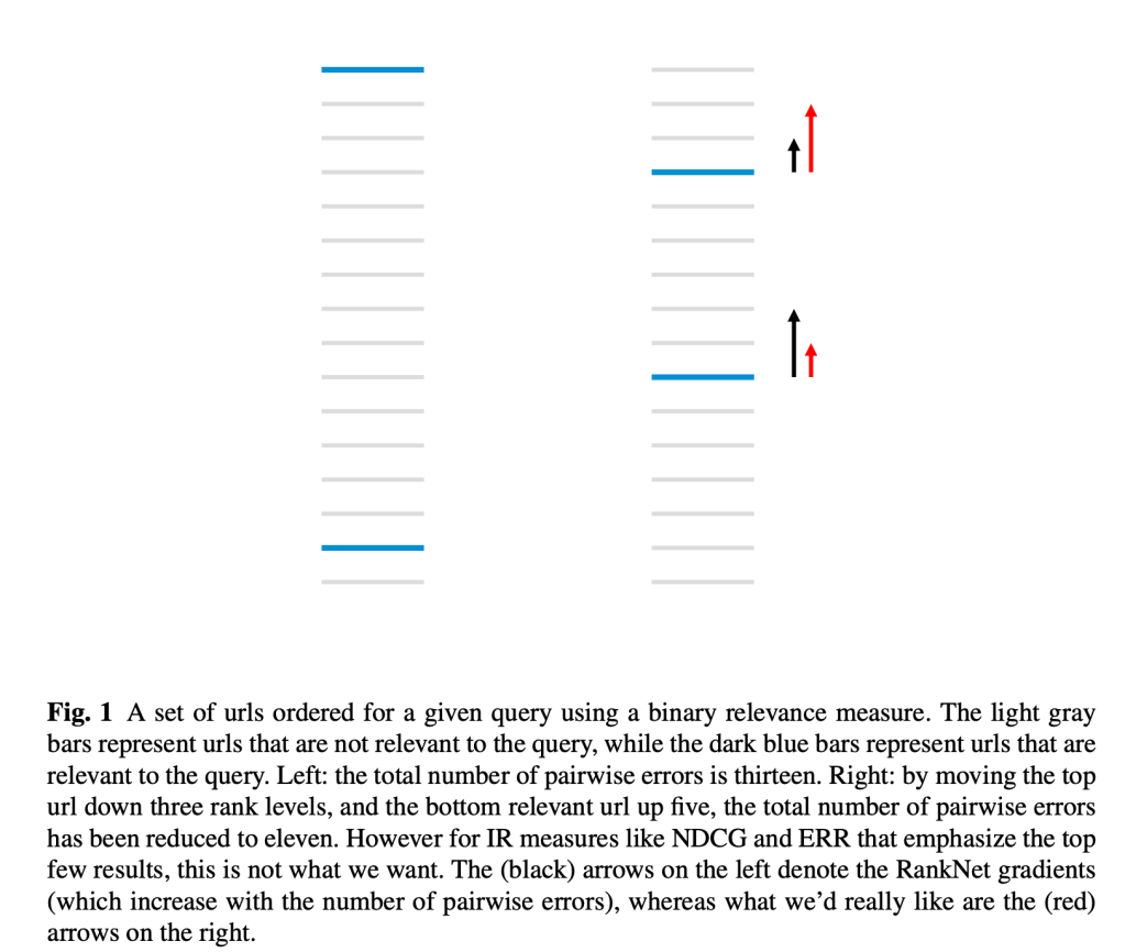
LambdaRank
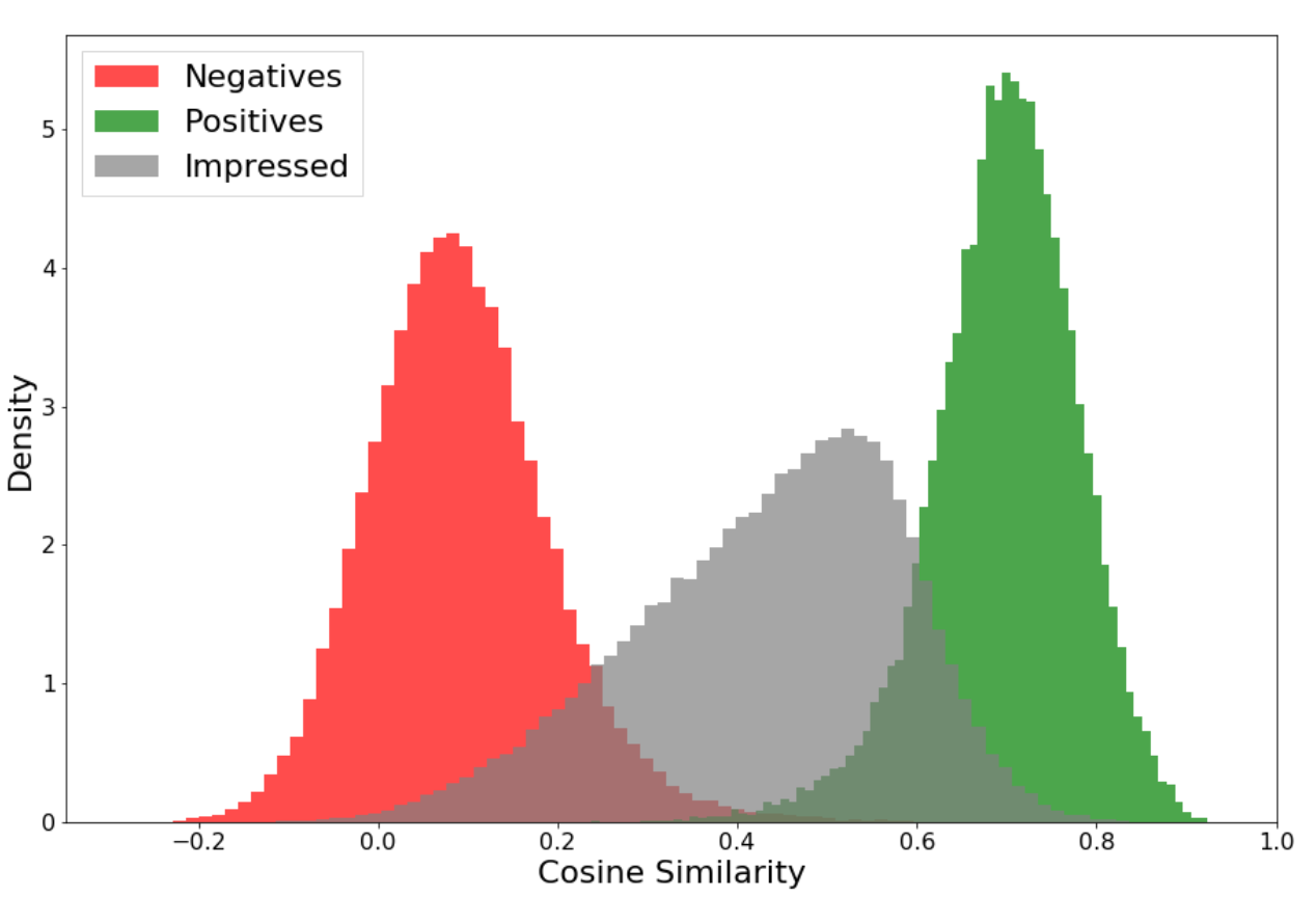
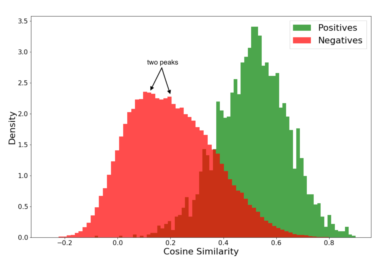
Figure below and caption explains why reducing pairwise difference does not necessarily results in increase of IR metrics. And LambdaRank is a way to optimize for IR metrics faster.
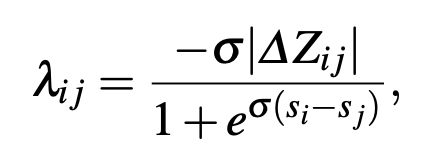
LamdaRank modified lamda_ij equation empirically as follows and it seemed to work well. We could do this because we don’t need to know actual cost function as long as we compute lamda_ij and then lamda_i
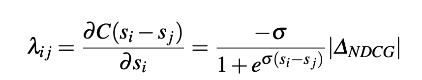
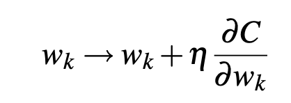
This becomes maximisation problem so we move in direction of gradient.
LambdaMART
- MART – Multiple Additive Regression. Trees. For more info read the post on gradient boosting
- To work with MART we need to specify two things
- Gradient of loss function, which will be used to fit the trees
- For the region in tree compute leaf value, that is done using line search/newton’s method
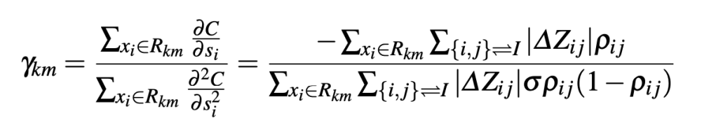
- We had empirically defined lambda as gradient in lambdaRank, we use same lambda as gradient here as well.
- For above lambda gradient, paper defines empirical cost function and then derives value at leaf nodes using newton’s method.
- Key difference to observe between lambdaRank and lambdaMART
- Lambda rank updates all weights (of classifier) after each query is examined
- Leaf value at lambdaMART is computed for all query, item pairs that falls into that leaf
- This allows lambdaMART to update splits and leaf values such that it may decrease utility for some queries but overall utility increases.
Reference
[0] : https://www.microsoft.com/en-us/research/blog/ranknet-a-ranking-retrospective/
[1] : https://www.microsoft.com/en-us/research/uploads/prod/2016/02/MSR-TR-2010-82.pdf