- Paper is related to search systems for e-commerce.
- It tries to replace BM-25 inverted index based recall with query-item embeddings.
- It is written by team at Amazon
- Paper URL – https://arxiv.org/pdf/1907.00937.pdf
- Shortcoming of BM-25
- lack of understanding of hypernyms, synonyms, antonyms
- hypernym – general/broad word
- Color is hypernym for red
- Examples
- Red dress and burgundy dress
- sneakers and running shoes
- Morphological variants (woman vs women)
- Stemming and lemmatization is typical solution
- Requires numerous hand-crafted rules
- Converts reading glasses to reading glass
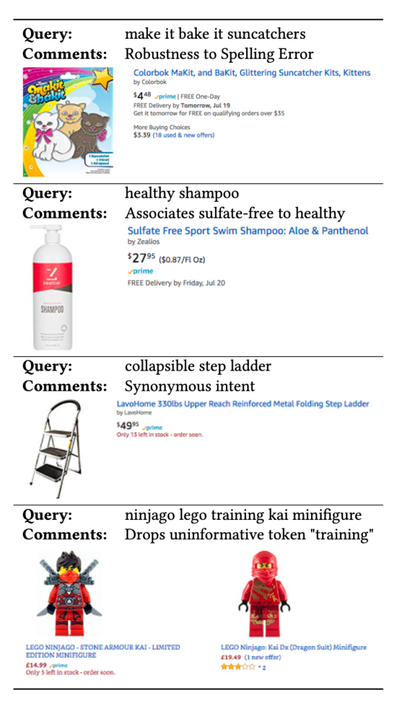
- Sensitivity to spelling error
- Typically solved by spell correction algorithms
- lack of understanding of hypernyms, synonyms, antonyms
Architecture
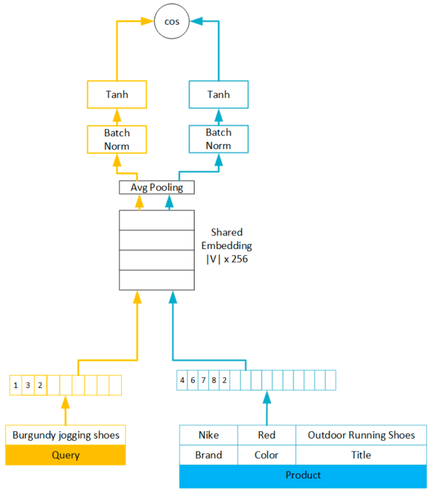
- Sharing embedding layer in siamese network work well, capturing local word level matching even before training this network.
- Average pooling
- Comparing to LSTM performance of average pooling reduced by just 0.5 %
- Evaluation metric were MAP and Recall@100
- It helped computationally
- Unlike web search query and items titles have smaller length
- Query also does not have stop words
- Batch Normalisation
- Length of items are generally longer than query
- They had observed difference in magnitude after avg pooling of query and item
- I have seen people using FC layer instead to have separate parameters
Loss Function
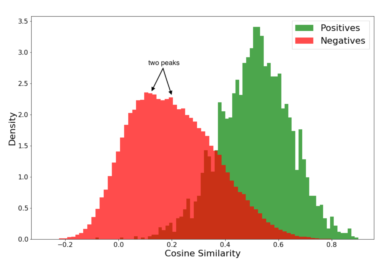

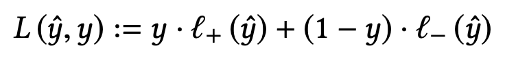

- They first tried with 2 part hinge loss
- Analysing the overlap items they found that they were clicked but not purchased.
- They note that from matching standpoint these products are okay to show to customer
- So they introduced third term and decided it’s threshold to be 0
- EmpIrical values used episolon (+) = 0.9, episilon (-) = 0.2
- My view on this
- For the products that has clicks but not orders, new loss tries to keep it below 0.55
- 2 part hinge loss was for purchased vs random items
- Some of those random items had got clicks
- For positive items when we get similarity above 0.9 it should contribute 0 to loss
- For negative items if we get similarity below 0.2 it should contribute 0 to loss
- For neutral items if we get similarity below 0.55 it should contribute 0 to loss
- y_hat is cosine similarity
- Based on which loss is calculated
- Instead of passing cosine similarity to sigmoid they are passing it through hinge function.
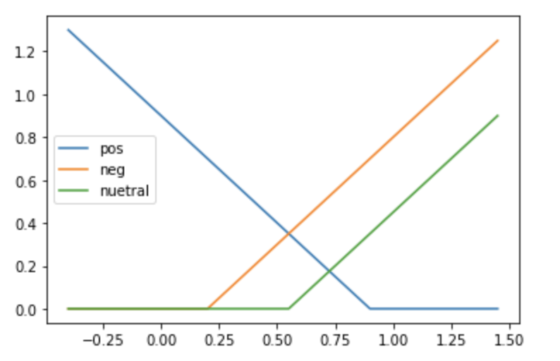
Tokenization Methods
- Word unigram
- word n-gram
- To preserve information about word ordering
- They preferred word n-gram over LSTM or CNN
- Character trigram
- Robust typos (iphone & iphonr)
- Compound words (amazontv & firetvstick)
- Item parts and sizes
- Tires have different sizes
- TVs have different model
- Handling unseen words
- Common NLP techniques
- Mask the input
- use same embedding for all unseen words
- What they choose
- Keep more embedding space for unseen words
- Hash them to get the bucket
- Enough space is allocated for frequent words and they are not hashed
- 10k or 100k of n-grams are kept
- Common NLP techniques
- Combining tokenization
- One approach
- Separate embedding for unigram, biagram and character trigrams
- Compute. weighted sum of cosine similarity individually
- Their approach
- Consider them as bag or words
- One approach
Data
- Time range
- Training data – 11 month
- Eval data – 1 month
- Trick of aggregating count as weight
- Weight while computing the loss, simple multiplication ( I had done that in synonyms as well )
- 54 billion query product training pairs
- Reduced to 650 million
- Ratio
- 1 purchased
- 6 impressed
- 7 random
- They plan for both matching and ranking
- Matching -> Differentiate between (purchased + impressed) from random
- Ranking -> Differentiate between purchased and impressed
- Query Preprocessing
- Changes queries to list of token IDs
- array length = 99 % tile of query token length
- Smaller tokens are padded to right
- Item preprocessing
- One approach
- Embed every attribute independently and concat
- Their approach
- Ordered Bag of words for title and attributes
- Issue was variability in attributes and lack of structured data across items
- One approach
Model Evaluations
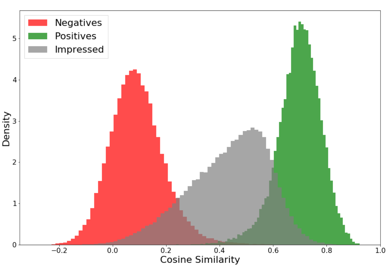
Evaluation Metrics
- Matching
- Recall@100 and MAP
- Used for tuning model hyper parameter as well
- 20k queries and sub-corpus for those queries
- Around 1M items
- Ordered + Impressed + Random
- Recall@100 and MAP
- Ranking
- NDCG and MRR
- Purchased + Impressed
Evaluation Results
- Table 1
- L2 variant of hinge loss outperforms L1
- They hypothesise that L2 is more robust to outliers
- 3 part hinge loss outperforms 2 part in matching but not in ranking
- Introduction of 3rd part forced purchased and random to be more separated
- L2 variant of hinge loss outperforms L1
- Table 2
- LSTM, GRU vs avg Pooling for aggregation
- Comparison is made for various losses
- Average pooling is performing similar or slightly better
- Definitely reduces computation time
- Since query and product title are relatively short this works well
- Recurrent methods are expressive but introduces specialisation between query and title
- Some may argue it is a good thing
- They argue that it might not capture local word level mapping
- LSTM, GRU vs avg Pooling for aggregation
- Table 3
- Compares different tokenization methods
- Vocab sizes in embedding space
- 125k – unigram
- 25k – bigram
- 64k – character trigram
- 500k – Out of vocabulary (OOV) bins
- Advantage of adding bigrams
- Example – Chocolate milk vs milk chocolate
- Advantage of character trigrams
- Robustness to spelling error
- OOV adds additional parameters
- case 1 : 500k unigrams
- case 2 : 125k unigrams and 375k OOV
- case 2 performs better
- Table 4
- Batch vs layer vs no normalisation
- query sorted data vs shuffled data
- Optimum combination was using batch normalisation with shuffled data
- Query sorted data did not have much effect on layer normalisation but was on batch normalisation
- Batch estimates for mean and variant would be biased for batch normalisation
- Table 5
- Comparing with baseline papers
- DSSM
- Learning Deep Structured Semantic Models for Web Search using Clickthrough Data
- https://posenhuang.github.io/papers/cikm2013_DSSM_fullversion.pdf
- ARC-II
- Convolutional neural network architectures for matching natural language sentences
- https://dl.acm.org/doi/10.5555/2969033.2969055
- Match Pyramid
- Text Matching as Image Recognition
- https://arxiv.org/pdf/1602.06359.pdf
- Two variation of their approach
- Frozen embedding
- Using pretrained word2vec and glove
- Randomly initialised embedding
- Lead 3X improvement in Recall@100 and MAP
- Frozen embedding
- DSSM
- Comparing with baseline papers
Online evaluations
- Three categories
- toys and games, kitchen and pets
- Conversion rate, revenue and other KPI increased with statistical significance
- Challenges
- Precision was decreased
- To mitigate they added guardrails using some heuristic and ranking models to filter non relevant items
- Not that recall@100 was metric for matching task and not precision.
Training Acceleration
- Increasing query product pairs from 200 million to 1.2 billion had improved matching metric by 10 %
- Data parallel training
- Idea
- Split data
- Same model on multiple GPUs
- Take the average of gradient in the end
- Cons for this architecture
- Limits embedding metric
- It has to fit on single GPU
- Data parallel approach has high communication overhead
- We need to weight till forward pass from each GPU is available
- Limits embedding metric
- Idea
- Model parallel training
- Pros in this architecture
- Simplicity of average pooling
- Siamese has some parallelism by default
- How they implemented
- Embedding metric is split across GPUs, across embedding dimension
- Hence we need to concat to get final embedding vector for each token
- Concatenation requires O(2k) communication of floating point numbers
- Partial token embeddings are averaged at each GPUs
- Hence we need to concat to get final embedding vector for each token
- Full dataset is sent to all GPUs
- Embedding metric is split across GPUs, across embedding dimension
- Pros in this architecture
- In the result section they have told that embedding dimension was 256
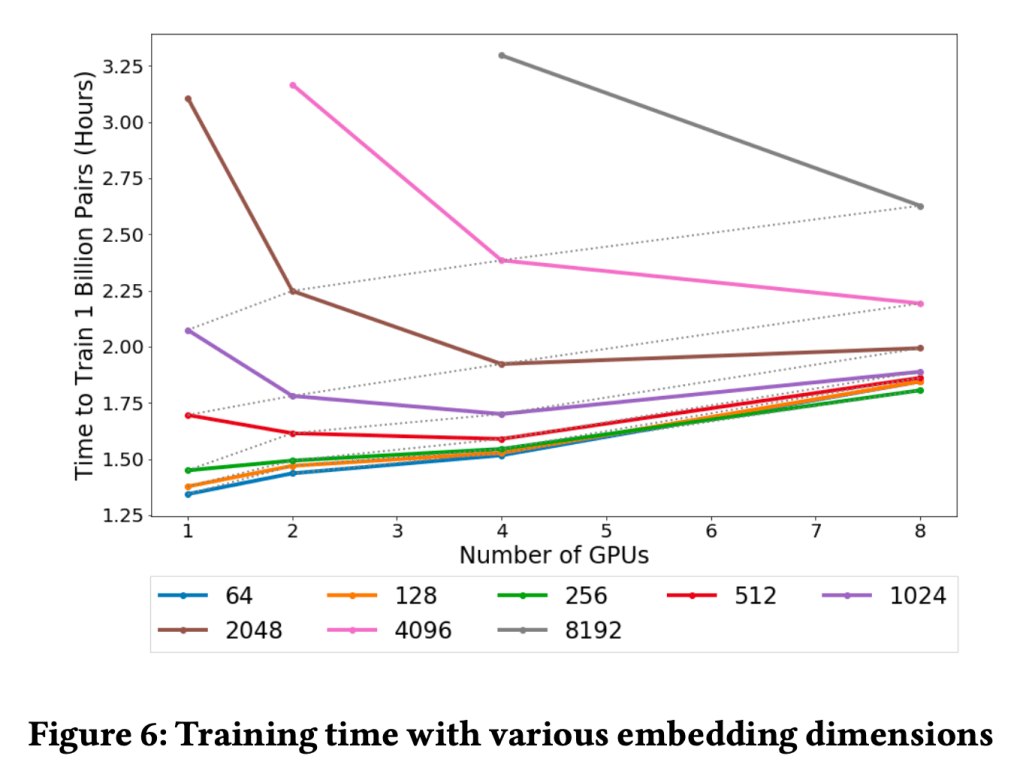
- Explaining above image
- For low embedding dimension time-to-train increases with number of GPUs but for high embedding dimension time-to-train decreases with number of GPUs
- Dotted line
- Following two should have same training time
- 2048 embedding with 1 GPU
- 1024 embedding with 2 GPU
- Doted line is for the ration of embedding_size/GPU
- With ideal scaling it would be horizontal
- Following two should have same training time
Exampels