Exponential, Poisson and Gamma Distribution

All three distribution models different aspect of same process – poisson process.

Poisson Distribution

  • It is used to predict probability of number of events occurring in fixed amount of time
  • Binomial distribution also models similar thing
    • No of heads in n coin flips
    • It has two parameters, n and p. Where p is probability of success.
  • Shortcoming of binomial
    • We want a single number i.e. k events per hour. Binomial has two – n & p
    • More than one event can occur in unit time. 1 like per hour, 1 like per minute.
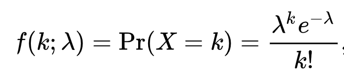
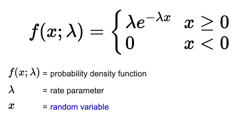
  • Below formula
    • lambda events occur in unit time
    • Below PDF is probability of k events in unique time
  • Properties
    • Popularly it is used to model rare events so we see small values of lambda often. But that is not restriction
    • Distribution is asymmetric. There is no such thing as # of events < 0
    • As lambda increases, it looks like normal distribution.
  • Poisson Model Assumptions
    • Average rate of events per unit time is constant
    • Events are independent

Exponential Distribution

  • Poisson – prob (k events in unit time)
  • Exponential – Prob (Amount of time between events) = Prob(amount of time until first event)
  • lambda – # no of events in unit time
    • rate
    • same as poisson
  • Derivation from Poisson
    • Exponential CDF can be derived from Poisson PDF
    • Differentiating it gives exponential PDF
  • Memoryless property
    • P(T > (a+b) | P(a) ) = P( T > b )
    • When memory is require we use weibull distribution
      • Older the car, more likely break down
  • When memory is not required
    • Probability that next bus arrives in less than 10 minutes
    • Probability that server will run without restart for 10k hours
    • Time for cook to prepare potato chips (probability not at a point, some range always)
  • Geometric distribution is counter part of exponential in discrete space
    • Corresponding poisson counterpart is binomial distribution
    • No of throws required to observe heads
    • It is also memory less
  • It is monotonically decreasing distribution
  • Expected value = mean = 1 / lambda

Gamma Distribution

  • Exponential – wait time till first. event
  • Gamma – wait time till k events
    • Two params – k and lambda
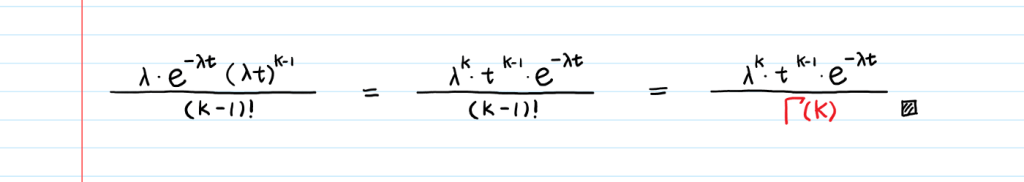
    • Probability of observing k events in time t
  • Applications
    • You are in a queue for medical checkup. There are 7 people in front of you. Avg time to check one person is 5 minute. (rate = lambada = 1/5 and k = 7)
  • Literature uses different symbols for above parameters
    • alpha, beta
    • theta, k
  • K can be real number in gamma distribution
    • To restrict k to be integer there is Erlang distribution
  • Gamma function – Gamma ( k ) = ( k – 1 ) !

Reference

Quantile Function (Inverse CDF)

Introduction

CDF maps input between in [0,1]. That is CDF(x) -> (0,1)

Quantile function takes input in (0,1) and return x.

  • Not all functionals are invertible.
  • Continuous distribution easily satisfies this property
  • For discrete distributions we take innfimum of all values [0]

Application in Sampling

  • Suppose we want to sample from a given distribution
  • We can make a quantile function of it
  • Sample uniformly from [0,1], call it p
  • x = quatile(p)
  • x is the sampled value [1]

Application in point estimation

  • Suppose you want to model CTR (click through rate)
  • CTR lies in (0,1) and can be presented via beta distribution
  • You have clicks and impressions for two ads/items anything
  • We are more confident about CTR when you have more impressions
  • We can construct a beta distribution with mean as point CTR.
    • ctr = beta(clicks, impression-clicks)
    • Recall in thompson sampling we were increasing alpha and beta by 1
  • Now we take 1%, 5%, 10% from quantile function. Call it
  • When we have more impressions ctr_x would be close to mean ctr (point estimate), else it will be less
  • On side node – this way of constructing distribution gets us away from point estimation and can be used in bayesian approaches

Reference

[0] https://stats.stackexchange.com/questions/212813/help-me-understand-the-quantile-inverse-cdf-function

[1] https://stats.stackexchange.com/questions/184325/how-does-the-inverse-transform-method-work/184337#184337

Central limit theorem

What does CLT says ?

  • Sum of random samples forms normal distribution
    • This samples may not come from normal distribution
  • Sum forming random distribution implies that mean would also form normal distribution

Straight facts

  • Central limit theorem helps getting confidence interval for parameters
  • It works for all distributions when n > 30
  • For normal distribution it works even if n < 30
  • Why do we need to have distribution
    • To make variance estimation stable
    • We want to have just one unknown that is mean
    • We need to test normality of samples before applying t-test

Slide from MIT course : https://ocw.mit.edu/courses/mathematics/18-650-statistics-for-applications-fall-2016/

sigma / (sqrt(n)) is standard error of mean. We are saying this distribution reaches to standard normal distribution.

Law of Larger Number

  • As a sample size grows, its mean gets closer to the average of the whole population. This is due to the sample being more representative of the population

Example:

  • During significance testing we calculate left hand side. For examples testing fairness of coin that number comes out to be 3.54. Now for standard normal 3*sigma = 3*1 = 3 is 99 % of area. We are further away than it. So we can reject null hypothesis. [1]
  • Thing to understand is that distribution of Bernoulli parameter(p) is normal.
  • We are not saying how far observed mean is from 0.5 in Bernoulli distribution. If we were doing that we would not have used sqrt(n).
    • Also more importantly Bernoulli can take only two values 0 and 1. From that perspective as well it does not make sense.
    • See the equation in the slide below in central limit theorem. It is a normal distribution N(0,1).

Refereces

[0] : Slide from MIT course : https://ocw.mit.edu/courses/mathematics/18-650-statistics-for-applications-fall-2016/

[1] : https://ocw.mit.edu/courses/18-650-statistics-for-applications-fall-2016/resources/mit18_650f16_parametric_ht/

Types of Statistical Studies

We study to learn something new. The word “study” in statistics implies conducting an experiment and analyzing data to learn something new, investigate something, or draw confident conclusions.

Studies are prevalent in medical fields, where people study various types of drugs on different demographics, geographies, and health conditions. This blog essentially contains my notes from the Coursera course: “Clinical Research” (https://www.coursera.org/learn/clinical-research/home/welcome).

Types of Studies:

  1. Observational Studies:
    • Case Series Study: Observes and describes subjects without requiring a research hypothesis. Numbers derived from such studies help remove inherent biases. These studies often serve as initial steps for complex studies.
    • Case Control Studies: Compare two or more groups based on the presence or absence of a disease. These studies look at historical data to identify variables that differ between the groups. Confounding, such as smoking in a study on alcohol and heart attacks, needs to be controlled for.
      • Many times when you are presenting analysis experienced seniors would ask what was the value of this feature in both cases ?
    • Cross-Sectional Studies: Conducted in the form of surveys, gathering data at a specific time. For example, a survey sent to optometrists and ophthalmologists to understand their dietary advice to patients. These studies aim to examine current practices and identify areas for improvement. (Reference: https://www.ncbi.nlm.nih.gov/pmc/articles/PMC3695797/)
      • Drawbacks
        • Responsive bias
          • Suppose you are asking questions related to HIV. Positive patients are less likely to answer than negative ones.
          • In govt survey people in cities are more likely to answer than villages
        • Almost impossible to infer causality
          • Since this takes place at a particular place in time, we can not determine whether disease outcome followed exposure or exposure followed disease.
    • Cohort Studies: Identify a group of subjects (cohort) and follow them either backward in history (retrospective cohort) or forward in the future (prospective cohort). Computerized data collection has made retrospective cohorts possible. These studies are observational and do not involve controlling variables.
  2. Experimental Studies (Interventional):
    • In these studies, interventions are implemented to reduce bias inherent in observational studies. There is a control group that receives no intervention (sham/placebo).
    • Some Key Terms:
      • Randomization: Every member of the population should have an equal opportunity to be part of the study, and participants should have an equal chance of being assigned to any group.
      • Blinding: Participants are unaware of their assigned groups. If researchers are also unaware of the groups, it is called a double-blind study. Achieving double-blindness is challenging in surgical operations.

Reservoir sampling

Where it is used

  • Suppose you have a streaming data and you want to randomly sample from it. You don’t know how many items will be coming in.
  • You have large set of items to sample from and you want to do it in single pass

How it is done

  • Suppose you want to sample 1000 items.[1]
  • You take first 1000 items and put it into reservoir
  • Next you will take 1001th item with probability 1000/1001
    • You take a random number and if it is less than 1000/1001, you add this item to reservoir
    • Remember the CDF trick
  • When you add this item, you randomly remove any other item from reservoir

Alternative

  • Pick items from stream, generate a random no and put it in priority queue
  • This is how order by rand() in sql works [1]

References

[1] https://gregable.com/2007/10/reservoir-sampling.html

[2] https://www.youtube.com/watch?v=Ybra0uGEkpM (proof)

Correlation and Regression Slope

In a simple regression model, the regression slope (β) represents the estimated change in the dependent variable (Y) corresponding to a one-unit increase in the independent variable (X). It quantifies the linear relationship between X and Y and indicates the direction and magnitude of the relationship.

The correlation coefficient (r) measures the strength and direction of the linear relationship between X and Y. It ranges from -1 to +1, with a value of 1 indicating a perfect positive linear relationship, -1 indicating a perfect negative linear relationship, and 0 indicating no linear relationship.

When the standard deviations of both X and Y are equal (SD(X) = SD(Y)), the regression slope (β) and the correlation coefficient (r) coincide.

The slope can be calculated as the correlation coefficient multiplied by the ratio of the standard deviations (β = r * SD(Y) / SD(X)). The correlation coefficient essentially represents the slope you would obtain from a regression of standardized variables (Y / SD(Y) on X / SD(X) or vice versa).

However, when the standard deviations of X and Y are not equal, the regression slope and the correlation coefficient provide distinct information:

  1. The correlation coefficient is a bounded measure that can be interpreted independently of the scale of the variables. It indicates the strength of the linear relationship between X and Y, with values closer to ±1 indicating a stronger linear relationship. The regression slope, on its own, does not provide this information.
  2. The regression slope represents the estimated change in the expected value of Y for a given unit increase in X. It provides information about the direction and magnitude of the relationship between X and Y in the original units of measurement. This information cannot be deduced from the correlation coefficient alone.

One more thing to add here is the relationship between correlation coefficient and co-variance. Formula is : r = Covariance (Y, X) / [ SD(Y) * SD(x) ]. We are normalising by SD of each variable. Also SD = sqrt ( variance ). We can also say that b = Covariance(X,Y) / VAR(X)

References

[0] : https://stats.stackexchange.com/questions/32464/how-does-the-correlation-coefficient-differ-from-regression-slope

[1] : https://www.quora.com/Is-there-a-relationship-between-the-correlation-coefficient-and-the-slope-of-a-linear-regression-line

VIF and Multicollinearity

VIF = Variance Inflation Factor

  • In linear regression collinearity can make coefficient unstable
    • There will not be any issue in prediction accuracy but coefficients would be less reliable and p-value would be more
    • Correlation coefficients help us detect correlation between pairs but not the multiple correlation x1 = 2*x3 + 4*x7
    • PCA is one thing, we don’t want to transform variable to keep interpretability intact
    • We want some way to reduce dimensions
  • In VIF, each feature is regression against all other features. If R2 is more which means this feature is correlated with other features.  [0]
    • VIF = 1 / (1 – R2)
    • When R2 reaches 1, VIF reaches infinity
  • We try to remove features for which VIF > 5

vif1

  • Example at [1] shows the use of VIF to reduce no of features.
  • Once we identify high VIF for features we need to reduce it
    • We can do it by eliminating some features
    • How to identify which feature to remove?
      • Check the correlated features for feature having high VIF
      • In the example at [1] weight and BSA were correlated
      • Practically it is easy to measure weight so we kept it
        • So such decision depends on the practical implication
      • There can be the case that one feature is correlated with many others and we might want to remove it      vif2vif2


Reference

[0] : https://www.youtube.com/watch?v=0SBIXgPVex8

[1] : https://newonlinecourses.science.psu.edu/stat501/node/347/


Chi Square Test

The chisquare independence test is a procedure for testing if two categorical variables are related in some population.

Here is handwritten example : https://github.com/arcarchit/datastories/blob/master/notes/chi2.pdf

Chi square distribution

  • Chi square distribution
    • Squaring samples from standard normal distribution [0]
    • Distribution changes with degrees of freedom
    • When DoF = 1 it is more concentrated around 0
  • It is distribution is sum of squares
    • When dice is biased sum of squares will be higher. Hence more significant.
    • When it is fair it will be closed to zero. Difference is with expected value.
d1
d2

Chi Square Test for Equality of Proportions

h1

Chi square vs T test

  • When to use which one
  • T-test is used to compare mean of two distributions
  • Chi square is used to check whether observation gathered of categorical data meets the assumption

Chi Square for goodness of fit testing

  • Chi Square Goodness of fit
    • Restaurant example
    • H0 = Percentage given by customer is correct
  • We calculate expected for each cell and calculate chi^2

Chi Square for relationship testing

  • H0 : Variables are independent of each other
  • It helps testing if two categorical variables are related
  • Calculate Chi square statistics by summing all cells and check against degree’s of freedom
  • Examples
    • Hypothesis testing :
      • H0 = Herbs1, Herb2, placebo are same
      • H0 = Herbs do nothing
      • We can’t say herb does nothing
        • We are working on accumulated data here
        • Whereas ANOVA is about variancei1
    • Homogeneity testing  :
      • H0 = Left and Right handed people have same preference for arts, science
      • H0 = Preference of arts/science is independent of natural hand left/right
      • H0 = Variables are independent
      • Filling up table
        • P(STEM | right) = P(STEM)
        • x / 60 = 40/100 => x = 40 * 60 / 100 = 24
        • We can also say that value of cell is product of marginals divide by total
      • Degrees of freedom = (r-1)*(c-1)  = 2 * 1 = 2
i3

References

[0] : https://www.khanacademy.org/math/statistics-probability/inference-categorical-data-chi-square-tests#chi-square-goodness-of-fit-tests

[1] : https://www.khanacademy.org/math/statistics-probability/inference-categorical-data-chi-square-tests#chi-square-goodness-of-fit-tests

[2] : https://biology.stackexchange.com/questions/13486/deciding-between-chi-square-and-t-test

[3] : https://fhssrsc.byu.edu/SitePages/ANOVA,%20t-tests,%20Regression,%20and%20Chi%20Square.aspx

Contrast Analysis

  • At Hypothesis and T-Distribution we discussed about hypothesis testing. We had talked about one sample and two sample t test.
  • Contrast analysis is more general case of that.
  • It allows us to make comparison of combination of groups :
  • Can’t we combine them to form just two groups :
    • We want to preserve individual identity of group
      • Group with large no of samples should not dominate group with small no of samples
  • Examples
    • Groups for which the context at test matches the context during learning (i.e., is the same or is simulated by imaging or photography) will perform better than groups with a different or placebo contexts. [2]
    • Group 1 is different from Group 2-3-4
      • 3 types of smile vs 1 neutral [3]
    • Group 1 and 4 are different from group 2,3


contrast1       contrast2

  • Intuition behind formula of standard error
    • Sum of square of combined group is some of individual SoS when groups are independent
  • α should be equal to desired confidence (0.90, 0.95 etc). It is divided by two because it is two sided


Reference

[1] : http://www.youtube.com/watch?v=yq_yTWK4mNs

[2] : https://pdfs.semanticscholar.org/c0ba/1c28b0e120a459820bfb20d430fa442ebd96.pdf

[3] : http://www.onlinestatbook.com/case_studies_rvls/smiles/index.html

ANOVA Introduction

ANOVA (Analysis of Variance) is a statistical technique used to determine if there are significant differences between the means of two or more groups. It is an extension of the t-test, which is used for comparing means between two groups.

The key idea behind ANOVA is to assess whether the data in different groups come from the same distribution or not. It is based on the assumption that data within each group should have low variance, while the variances between the groups should be relatively high.

The null hypothesis in ANOVA states that the means of all the groups are equal. If the groups are well separated and one group appears to be significantly different from the others, the null hypothesis is rejected.

There are different types of ANOVA designs, including one-way ANOVA and two-way ANOVA.

One-way ANOVA involves comparing the means of a single dependent variable across three or more independent groups. For example, you can use one-way ANOVA to analyze the stress levels of employees before the layoff announcement, after the announcement, and during the layoff period.

Two-way ANOVA, on the other hand, involves examining the interaction effects between two independent variables on a dependent variable. For instance, you can use two-way ANOVA to explore the stress levels of men and women before the layoff announcement, after the announcement, and during the layoff period. In two-way ANOVA, there are multiple null hypotheses to test, including whether the stress levels are the same for men and women, whether the stress levels are the same across different time points, and whether there is an interaction effect between gender and time.

The F distribution is utilized in ANOVA, similar to how the t distribution is used in t-tests. The F distribution has different shapes depending on the degrees of freedom for the numerator and denominator. As the degrees of freedom increase, the F distribution becomes more concentrated. It ranges from 0 to infinity, denoted as [0, infinity).

I have coded a notebook for calculating one way anova manually in python [1]

ANCOVA, MANOVA, MANCOVA

ANCOVA (Analysis of Covariance), MANOVA (Multivariate Analysis of Variance), and MANCOVA (Multivariate Analysis of Covariance) are related techniques.

ANCOVA (Analysis of Covariance) is an extension of ANOVA that incorporates a continuous independent variable, referred to as a covariate. The purpose of ANCOVA is to examine whether the relationship between the dependent variable and the independent variable(s) remains significant after controlling for the effect of the covariate. By including the covariate in the analysis, ANCOVA allows for a more accurate assessment of the impact of the independent variables on the dependent variable.

MANOVA (Multivariate Analysis of Variance) is used when there are two or more dependent variables. It examines whether there are significant differences between groups across the multiple dependent variables. MANOVA allows for the analysis of complex relationships among variables and provides a comprehensive assessment of group differences. It is particularly useful when the dependent variables are related or correlated.

MANCOVA (Multivariate Analysis of Covariance) is an extension of MANOVA that incorporates continuous independent variables along with the categorical independent variables. MANCOVA allows for the examination of the effects of both categorical and continuous independent variables on multiple dependent variables while controlling for the influence of covariates. It helps to determine whether the relationships between the independent variables and the dependent variables remain significant after accounting for the effects of covariates.

In summary:

  • ANOVA is used to compare means between three or more groups.
  • ANCOVA extends ANOVA by incorporating a continuous covariate to control for its effect.
  • MANOVA analyzes differences between groups across multiple dependent variables.
  • MANCOVA extends MANOVA by including both categorical and continuous independent variables along with covariates.

These techniques are widely used in research and can provide valuable insights into group differences and relationships among variables.

References:

[0] : https://www.technologynetworks.com/informatics/articles/one-way-vs-two-way-anova-definition-differences-assumptions-and-hypotheses-306553

[1] : https://github.com/arcarchit/datastories/blob/master/ANOVA.ipynb

[2] : http://www.statsmakemecry.com/smmctheblog/stats-soup-anova-ancova-manova-mancova