Anomaly Detection Basics

These are notes form Andrew N.G’s machine learning course on coursera.

Anomaly Detection Problem

  • Assembly line prepared aircraft engine, you want to check if it okay.
    • Features can be
      • heat generated
      • vibration intensity
  • Fraud detection in finance/retail
    • Feature would be based on user’s activity
  • Monitoring CPUs in data center
    • Features would be memory used, CPU load, network traffic.
  • Generally we have less number of positive (anomalous example) compared to negative ones (normal).

Solution Based on density Estimation

  • We try to fit normal examples in gaussian distribution
  • For new engine we estimate the probability of it p
  • If p < epsilon – we flag the new engine as anomalous
  • We generally train one gaussian per features and multiply like naiver bayes
    • That is to say off diagonal elements in multivariate gaussian are zero
    • More details in the last section of this post ( multivariate gaussian )

Model Evaluation

  • Once we have multiple models having different features how to evaluate which one is better ?
  • We also need to tune epsilon parameter.
  • We can use standard setup of train-set, test-set and cross validation set
  • Train set would have normal examples only. It would okay if few anomalous samples slips in
    • So training is unsupervised only
    • Predict y = 1 if p(x) < epsilon else 0
  • Bad metric
    • classification accuracy (because classes are imbalanced)
  • Good metric
    • TP, FP, TN, FN
    • Precision/recall
    • F1 score
  • Cross validation set is used for tuning epsilon

Anomaly Detection vs Supervised Learning

  • Supervised model like logistic regression would require
    • 1) More training examples
    • 2) Somewhat balanced classes

Feature Engineering

  • Since we are fitting gaussian we need to do some transformation if feature distribution does not look like one. Popular transformations are
    • log (x)
    • log (x + c)
    • sqrt (x)
  • How to introduce new feature
    • We need to do this when p(x) is comparable for normal and anomalous sample
    • Once you find anomalous sample for which p(x) is not low enough, try looking deep into it.
    • Property which is making it anomalous would be a new feature to add
  • Feature Engineering Recommendation
    • Think about features which will be too high or too low in case of anomaly
    • x5 and x6 can be a good feature in below image.

Multivariate Gaussian

  • Shortcoming of individual gaussian is that in case of correlated features it won’t be able to detect the anomaly.
    • Green sample in above image will not be detected
  • To mitigate this we can hand-code ratio based features
  • Original model is more popular because it scales well with no of features.

Clustering Metrics

Here are some metric available for validating clustering, explanation of each one is available on sklearn. [0]

If ground truth labels are available:

  • Adjusted Rand Index
  • Mutual Information Based scores
  • Homogeneity, completeness and V-measure
  • Fowlkes-Mallows scores

If not available :

  • Silhouette Coefficient
    • Range (-1,1)
    • 1 means it is similar to data-points in each cluster
  • Calinski-Harabaz Index
  • Davies-Bouldin Index
  • Contingency Matrix


Calculating SSE

It is a sum of distance between each point and its cluster center.

c1

Silhouette Score

It is calculated for each point and then we take an average of it.

c2

c4           c3

a(i) is average distance of a point to other points in same cluster.

b(i) is minimum of above average in for point in other cluster. It given the distance to nearest cluster.

s(i) close to 1 means data point is appropriately clustered. -1 means it is very bad clustered.

Setting s(i) to 0 when cluster size is one ensures that curve is not monotonically decreasing.


Elbow method and Silhouette Analysis

Notebook is available at https://github.com/arcarchit/datastories/blob/master/Silhouette.ipynb

sil1         sil2

Rand Index

  • When cluster labels are available we can use this matrix
  • It basically checks the similarity between two cluster assignments
    • Labels can also be seen as one type of cluster assignment
    • Score basically tells us how similar to cluster assignments are
  • This works by taking pair of points
    • Out of all pairs how many pairs are agreed in both clusters mechanism
    • Agree mean both
      • They are in same cluster in both mechanism
      • They are in different cluster in both mechanism
  • The Rand index has a value between 0 and 1, with 0 indicating that the two data clustering do not agree on any pair of points and 1 indicating that the data clustering are exactly the same

rand_index

  • One drawback of Rand index is that it can given non zero value for random assignment of clusters. To mitigate that there is matrix called Adjusted Rand Index. [2]
    • It specifically does not work when no of clusters are high


Reference

[0] : https://scikit-learn.org/stable/modules/clustering.html

[1] : https://github.com/anthonyng2/udemy-the-complete-machine-learning-course-with-python

[2] : https://davetang.org/muse/2017/09/21/adjusted-rand-index/


Hidden Markov Models

From a Clustering Perspective

This section summarizes a lecture from the University of Washington [0] on clustering time series data, considering the significance of both the data and indices.

Other potential applications include:

  1. Honey bee dance: Bees switch from one dance to another to convey messages.
  2. Conference conversations: Segmenting speaker assignments based on the spoken turns.
  3. Gym exercises: Identifying exercises from pulse rate data as people switch between activities.

Model

The following screenshots are from a YouTube video [1] by the Mathematical Monk, illustrating the model:

Suppose you’re developing handwriting recognition and need to recognize a hidden variable.

The prediction for “i” depends solely on the previous character being “h,” disregarding how “h” was written.

hmm_concept
hmm_parameters

Code and Notebook

You can find the code and notebook at the following GitHub link [2], which extensively explains:

  1. The structure of the model.
  2. The forward algorithm for calculating the likelihood of a given observation.
  3. The backward algorithm for finding the most probable state sequence given an observation (also known as decoding).
  4. The forward-backward algorithm for inferring model parameters from a set of observed sequences.

References

[0] : https://www.coursera.org/learn/ml-clustering-and-retrieval/home/welcome

[1] : https://www.youtube.com/watch?v=TPRoLreU9lA

[2] : https://github.com/arcarchit/datastories/blob/master/hmm.ipynb

[3] : https://web.stanford.edu/~jurafsky/slp3/A.pdf

Hierarchical Clustering

This post is a lecture summary of  course by University of Washington : https://www.coursera.org/learn/ml-clustering-and-retrieval/home/welcome


Why one might want to use hierarchical clustering ?

  • A common problem is clustering is to predefined no of clusters (k)
    • Hierarchical clustering does not need that
  • Deprogram provides effective visualization of clusters at various levels without re-running the algorithm
  • Any distance metric can work, while k-mean required euclidean distance [0][1]
  • We can construct more complex shape compared to k-means/EM


Divisive clustering

  • Example algorithm is recursive k-mean
  • We first cluster with k = 2 and then recursive apply k-means on these two clustersdivisive_clustering
  • Various choices we need to make :
    • Which algorithm to use (k-means)
    • How many split at each level (k=2, 3)
    • When to stop? Here are some heuristics:
      • Number of points in a cluster falls below certain threshold (Minimum point in each cluster)
      • Distance to farthest point falls below certain threshold (Minimum cluster radius)
      • Until per-specified no of clusters are reached


Agglomerative clustering

  • Example would single linkage algorithm
  • We start with assigning each point to its own cluster
  • Next task is how to merge this cluster
    • How do we define the distance between cluster?
      • Linkage function
        • It gives us two points from each cluster
        • Single linkage given points which has minimum distance across all possible pairs
        • Cluster A has points (a1, a2, a3) and B has (b1, b2, b3)
        • Linkage will give say (a2, b3) if it has the minimum distance across all combination
      • Distance Function
        • Can be euclidean or cosine anything
    • We merge the cluster which has minimum distance
  • Dendrogram provides efficient visualization [4]
    • Data-points of x-axis carefully ordered
    • Height (y-axis) represents distance between two cluster as per specified linkage
    • It gives us the complete visualization of which nodes were merged first followed by which one etc.
  • How to cut dendrogram ? [4]
    • Suppose we are cutting the dendrogram at y=D*
    • There are no pair of cluster which has distance < D* and which is not merged
    • All the pairs of clusters having distance < D* are merged
    • D* is the minimum distance between cluster at this level
    • Distance between clusters identified > D*
  • Various linkage functions [2][3]
    • Complete linkage takes two farthest points
    • Average linkage considers all pairs and takes an average
    • Ward linkage focus on increasing sum of squares
    • These linkage however brings down the shaping flexibility
      • Single linage would allow for complex shapes in general
      • Single linkage however can result in chaining
  • Choice we need to make in agglomerative clustering
    • Which linkage function to use
    • Which distance metric to use
    • Should we cut dendrogram flat or some weird cut

dendrogram

  • Complexity
    • For brute-force it is O(N^2 log N)
    • We can also prune search space by kd-trees or using triangular inequality
    • Best know is O(N^2) [5]


Linkage Functions

linkage

References

[0]: https://stats.stackexchange.com/questions/81481/why-does-k-means-clustering-algorithm-use-only-euclidean-distance-metric

[1]: https://pdfs.semanticscholar.org/a630/316f9c98839098747007753a9bb6d05f752e.pdf

[2] : https://www.saedsayad.com/clustering_hierarchical.htm

[3] : https://stats.stackexchange.com/questions/195446/choosing-the-right-linkage-method-for-hierarchical-clustering

[4] : http://www.econ.upf.edu/~michael/stanford/maeb7.pdf

[5] : https://www.cs.ucsb.edu/~veronika/MAE/summary_SLINK_Sibson72.pdf

Probabilistic Clustering

This post serves as a lecture summary of a course offered by the University of Washington, which can be accessed at the following link: University of Washington – ML: Clustering and Retrieval.

Sample code related to the course can be found on GitHub at: Sample Code for EM Algorithm.

In this lecture, we will cover several important topics:

  1. Why we need probabilistic clustering: We will explore the motivations behind using probabilistic clustering methods, which allow for soft assignments to clusters rather than rigid assignments.
  2. Mixture models: We will dive into the concept of mixture models, which are a probabilistic approach to clustering. Mixture models allow data points to belong to multiple clusters with different probabilities.
  3. Expectation Maximization (EM): We will study the Expectation Maximization algorithm, a powerful iterative algorithm used to estimate the parameters of mixture models. EM alternates between the expectation step, where cluster assignments are updated based on current parameter estimates, and the maximization step, where the parameters are updated based on current cluster assignments.

Why we need probabilistic clustering ?

To understand the need for probabilistic clustering, let’s consider the problem of determining user preferences based on their feedback. Suppose users provide feedback on whether they liked or disliked an article. We want to gather this feedback and group it into clusters to gain insights into their preferences.

For instance, imagine a user who likes an article about the first human landing on Mars. This article could be relevant to both world news and science news categories. In such cases, assigning articles to clusters with a hard assignment (where an article belongs to only one cluster) may not capture the complete picture. Soft assignment to clusters, where an article can belong to multiple clusters with different probabilities, is more suitable.

Now, let’s explore some scenarios where the traditional K-means algorithm fails:

  1. Clusters with Different Spreads: When clusters have varying spreads, simply deciding based on a single sample may not provide an accurate representation. Instead, it is important to consider the number of data points within each cluster. Assigning an ambiguous point to a cluster that has more data points can be a more meaningful approach.
  2. Overlapping Clusters: In cases where clusters overlap, soft assignment becomes crucial. It allows for assigning data points to multiple clusters based on the degree of membership.
  3. Clusters with Different Shapes or Orientations: When clusters have distinct shapes or orientations, measuring the distance to the cluster center alone is insufficient. Considering the shape of the clusters is necessary for accurate clustering.

One approach to address these challenges is using K-means with scaled Euclidean distance. This modification results in clusters represented by axis-aligned ellipses, accommodating different spreads in each dimension. However, determining appropriate weights for each dimension in the calculation remains a question that needs to be addressed. Shape is still axis-aligned ellipses, which is a limitation in itself.

Motivating application

Let’s consider the task of clustering images based on their color composition. One approach is to compute the average values of the red (R), green (G), and blue (B) channels for each image. This results in representing each image as a single 3-dimensional vector [R, G, B], capturing the average color values.

By applying clustering algorithms to these image vectors, we can group similar images together based on their dominant color characteristics. Although our data is unlabeled, we can observe potential clusters such as:

  1. Sky Cluster (Blue Dominated): Images that predominantly contain blue colors, such as those depicting clear skies, can be grouped into this cluster.
  2. Sunset Cluster (Red Dominated): Images showcasing vibrant sunsets with warm hues and red tones can be grouped into this cluster.
  3. Forest Cluster (Green Dominated): Images featuring lush green forests, landscapes, or vegetation will likely be grouped into this cluster due to their dominant green color composition.

Mixture Models

  • Here is how distribution of blue might look for all images
blue

We can model image clustering using a mixture of Gaussian distributions. The model consists of three Gaussian components, each with its own parameters (μ and σ). The final distribution is a convex combination of these components: π1g1 + π2g2 + π3*g3, where 0 ≤ π ≤ 1 and the sum of all π values is equal to 1.

Each mixture component represents a unique cluster, characterized by its own set of parameters (πk, μk, σk). In the case of multidimensional data, such as image vectors, each individual distribution is a multivariate Gaussian distribution.

Without examining the image vector, we can determine the probability of it belonging to cluster k using the πk value. Given an image vector x, we can estimate the probability of it belonging to cluster k as P(x | params) = P(x | μk, Σk), where Σ represents the covariance matrix in the multivariate Gaussian.

Clustering with soft assignment involves calculating a responsibility vector for each data point. The length of the responsibility vector corresponds to the number of clusters, which in this case is three (sky, forest, sunset). Each element of the responsibility vector represents the probability of a data point belonging to a specific cluster.

In the case of document clustering, where the dimensionality is high (proportional to the number of words in a vocabulary), keeping track of parameters for each Gaussian becomes computationally expensive. To address this, we simplify the model by considering only diagonal values in the covariance matrix, effectively restricting the model to axis-aligned ellipses. This approach is similar to K-means with scaled Euclidean distance, which also allows for axis-aligned ellipses.

However, the advantage of the mixture model is twofold:

  1. We do not need to specify weights for each dimension in advance; the model learns them from the data.
  2. Different clusters can have varying weights for each dimension, allowing for more flexible modeling of the data.

EM

Responsibility vector calculation with known cluster parameters

  • The responsibility vector can be calculated if we know the cluster parameters: π_k, μ_k, and ∑_k.
  • The responsibility vector is different from the π values.
  • Given a data point, we can find its corresponding responsibility vector by estimating the probabilities in that cluster.
  • The responsibility vector needs to be normalized after evaluating the probabilities.
a
  • This process is a consequence of Bayes’ rule.

Estimating cluster parameters with known responsibility vectors

  • It is similar to parameter estimation of a multivariate Gaussian.
  • Each data point, x_i, is multiplied, and there is no need to worry about the denominator since it is also not N (the number of data points).
  • b1         b2      nk_soft
  • N_k_soft implies how many points belong to cluster 1
    • Also it is a soft assignment

EM Algorithm

  • E-step: Estimation of the responsibility vector given parameters.
  • M-step: Maximum likelihood estimation of the parameters given the responsibility vector.
  • These two steps are repeated until convergence.
  • The EM algorithm can be derived as a coordinate ascent algorithm and converges to a local mode.
  • The biased coin example provides a good illustration of the EM algorithm. Check the image below

mj0nb

Challenges

  • The probability becomes infinite when the variance becomes zero.
  • This can occur when there is only one data point in a cluster, and the mean is itself with zero variance.
  • In high-dimensional spaces, this often happens, such as when a document does not have a specific word at all.
  • To solve this issue, a small value is added to the diagonal elements of the covariance matrix, similar to adding a prior in Bayesian approaches.

Relationship to K-means:

  • When a Gaussian has the same variance in all dimensions and shrinks to zero, the likelihood becomes either 0 or 1.
  • This behavior is similar to hard assignment, resembling the K-means algorithm.

Initialisation

  • Choose k observations at random and assign observations to nearest centroid
  • Above via k-means++
  • Solution of k-means
  • Grow mixture model by splitting cluster (sometime merging) until K clusters are formed

I have coded simple EM at [0]

References

[0] : https://github.com/arcarchit/datastories/blob/master/EM.ipynb

K-Means Clustering

This post is a lecture summary of a course by the University of Washington available on Coursera: Machine Learning: Clustering and Retrieval.

Application

We want to discover groups of articles (e.g., sports, world news) without knowing the labels in advance. We can assign labels after finding clusters. Our goal is to learn user preferences, whether she likes sports/technology etc.

Users provide feedback on whether they liked an article or not. We can accumulate this feedback within specific clusters to understand preferences.

Contrast this with building a classification model that predicts whether a user will like a specific article. For that, we would need to build a classifier for each user and score each (article, user) pair.

Alternatively, we can determine the types of articles each user prefers and show nearby articles using K-nearest neighbors (KNN). Clustering offers a more elegant and simplistic approach.

Unsupervised Task

Clustering is an unsupervised task since there are no input-output labels. Unsupervised learning poses challenges:

  • Defining clusters can be easy or hard, depending on the case.
  • Our algorithm works well for cases with intermediate difficulty.
  • There are still unsolved clustering problems.
unsolved_clustering

Clustering in General

A cluster is defined by its center or centroid and its shape, often represented by an ellipsoid.

K-Means

Scoring in K-means involves assigning a point to a given cluster. The scoring mechanism is the distance to the cluster center.

K-means alternates between two steps:

  1. Assign data to clusters.
  2. Update cluster centers.
step1
step2

Both steps are minimization steps, making K-means resemble a coordinate descent algorithm. We alternate between minimizing in two directions: μ (cluster assignment) and z (cluster center).

Convergence

K-means is a non-convex optimization problem, so the global minimum is not guaranteed. We aim to find zᵢ and μᵢ that minimize the objective function.

k_means_objective

By optimizing via coordinate descent, K-means can converge to a local minimum. However, convergence depends on the initialization. To improve convergence, we use smart initialization as described below.

Smart Initialization

  1. Pick the first center randomly.
  2. Calculate the distance to the nearest center for all data points.
  3. Choose the next center with a probability proportional to the squared distance.

To perform probability sampling, calculate the cumulative probability as described in [1]. When K-means is followed by this initialization, it is known as K-means++.

Trade-offs

K-means++ takes more time for initialization but converges faster. Additionally, the converged solution is better than that of regular K-means.

Assessing Quality

Quality can be assessed by evaluating the objective value after convergence, which is referred to as cluster heterogeneity. A smaller heterogeneity indicates a better algorithm. Tighter clusters are more homogeneous.

Beware of overfitting: as K increases, heterogeneity always decreases.

Choosing K

To choose K, you can heuristically plot heterogeneity for various values of K and select the one at the elbow. Alternatively, you can use hierarchical clustering, which doesn’t require specifying K in advance. We can also perform Silhouette Analysis.

References

[1]: Stack Overflow: How exactly does k-means++ work?

Nearest Neighbour Search


This post is a lecture summary of a course by the University of Washington available on Coursera: Machine Learning: Clustering and Retrieval.

Problem: Document Retrieval

Given a document, we want to search for similar documents in a corpus.

Representation: How to Represent Documents as Vectors?

  • Bag of Words: Count the frequency of each word in the vocabulary.
  • TF-IDF: Calculate the IDF (inverse document frequency) of each word in the vocabulary. Weight word frequency (TF) by its IDF in a given document.
    • TF: Same as bag of words.
    • IDF: Higher for rare words, calculated as log(D_total / (1 + D_word)).

Distance Metrics

There are different distance metrics used to measure similarity or dissimilarity between vectors. Let’s explore some commonly used distance metrics:

Euclidean Distance:

  • Euclidean distance between two vectors x and y can be calculated using the vectorized form: sqrt((x-y).T.(x-y)).
  • It is beneficial to normalize features because features can have different units and varying ranges.
  • Normalization can be achieved by dividing either by the range or by the variance of the features.

Scaled Euclidean Distance:

  • Scaled Euclidean distance allows for weighting different dimensions differently based on their importance.
  • For example, in text analysis, we may want to give more weight to the title/abstract than the body of an article.
  • This can be achieved by summing up the word vectors of the article and title and using a diagonal matrix A that contains weights for each feature.
  • The vectorized form for scaled Euclidean distance is: sqrt((x-y).T.A.(x-y)).

Cosine Similarity:

  • Cosine similarity measures the cosine of the angle between two vectors.
  • Similarity = x.dot(y).
  • Distance = 1 – similarity.
  • Cosine similarity is not a proper “distance” metric because it does not satisfy the triangular property (|ab| + |bc| > |ac|).
  • Cosine similarity is commonly used in Natural Language Processing (NLP) tasks due to its computational efficiency for sparse features.
  • Feature vectors in NLP tend to be sparse.
  • The range of similarity values is generally between -1 and 1. However, when features are non-negative, the range becomes 0 to 1, which is the case with TF-IDF.
  • Normalization can be performed instead of using the inner product: Similarity = x.dot(y) / (|x||y|).
  • Normalization avoids doubling the length of documents by copying.
  • One side effect of normalization is that long documents and tweets may appear similar, which is undesired when suggesting tweets to someone reading a document.
  • To address this, an alternative approach is to cap the maximum word count that can appear in a vector.

Cosine vs Euclidean:

  • The choice between cosine and Euclidean distance depends on the use case.
  • Cosine distance is more suitable for text features where the magnitude of the vector is not as important as the orientation.
  • Euclidean distance is a better choice for count features, such as measuring how many times a document was read.
  • For mixed feature types, both cosine and Euclidean distances can be computed (possibly with a subset of relevant features) and combined using appropriate weights, considering the trade-offs and requirements of the specific problem.


Brute Force

  • Calculate distance to each document in corpus
  • Suppose there are N documents in corpus
  • Complexity  would be O(N) for 1-NN
  • It will be O(N log k) for k-NN
    • Using priority queue
  • It is computationally inefficient when we N is large and we need to query often

KD-Trees

KD-Trees are used to divide the space into hierarchical regions via a tree structure. Here’s how it works:

  • At each node, we store the smallest bounding box that contains all the data points in that region.
  • While querying (for 1 nearest neighbor, which can be extended for k nearest neighbors):
    • First, we find the leaf node where the query point belongs.
    • Then, we find the nearest neighbor within that node.
    • We keep moving up in the tree.
    • If the distance between the query point and the bounding box is greater than the distance found so far, we skip that region and move up the tree.
    • If it is less, we traverse down the tree.
  • To calculate the distance between a point and a rectangle, you can use appropriate distance metrics like Euclidean distance or other suitable measures. It is computationally easy rectangles are axis aligned[1]

Construction of KD-Trees:

Here are the steps involved in constructing KD-Trees:

  • Choose a splitting strategy:
    • Widest dimension: Split based on the dimension with the widest range.
    • Alternating dimension: Split alternately between dimensions.
  • Determine the value to split on (split value):
    • Median: Choose the median value of the points along the splitting dimension.
    • Center point: Compute the center point as the average of the left and right extremes.
  • Stop conditions for splitting:
    • If there are fewer points left than a specified threshold.
    • If the minimum width of the region is achieved.

How to Prune More Aggressively:

To prune more aggressively in KD-Trees, consider the following approach:

  • Suppose the nearest distance found is r.
  • Instead of pruning points that are farther than distance r, prune all points that are farther than (r/a), where a > 1.
  • This allows for more aggressive pruning and can speed up the search process.

Limitations of KD-Trees:

KD-Trees face challenges in high-dimensional spaces. Here are some limitations:

  • In high dimensions, the radius of the search space is generally large.
  • For d dimensions, the radius intersects 2^d hypercubes, resulting in an extensive search space.
  • One possible solution is to prune all points that are farther away than (r/a), where a > 1, to mitigate these issues.


LSH – Locality Sensitive Hashing

Locality Sensitive Hashing (LSH) is a technique used to classify data points into various bins and search within a given bin. Here’s how it works:

  • The idea is to group data points into bins based on their proximity and search within the relevant bin(s).
  • If necessary, nearby bins can also be explored to expand the search.
  • To determine nearby bins, multiple random lines (or planes in higher dimensions) are used.
  • Let’s consider a motivating example with points in a 2D plane:
    • A single random line passing through the origin is chosen.
    • Points that are closer to each other will mostly fall into the same bin.
  • However, using just one line can lead to more data points in a single bin, increasing query time.
  • The solution is to use multiple random lines (or planes) to achieve more efficient classification of neighboring bins.
  • For example, let’s consider three lines, f1, f2, and f3, defined as f(x,y) = 3x + 4y = 0:
    • If f1(p,q) < 0, f2(p,q) > 0, and f3(p,q) > 0 for a given point (p,q), we assign it to the bucket [0,1,1].
  • To facilitate searching within bins, a dictionary can be used, where the key represents the bin (e.g., [0,1,1], [0,1,0]), and the value is a list of all points in that bin.
  • To find nearby bins:
    • Flip one bit to find bins with a single bit difference.
    • For more exploration, flip two bits to find bins with two bits difference.
  • It is possible for the nearest point to be in a different bin.
  • The number of neighboring bins to explore depends on factors such as computational budget or a predefined quality threshold.
  • In some cases, an exact nearest neighbor may not be necessary, and a point with a predefined quality (epsilon) is sufficient.
  • LSH is useful in scenarios like document suggestion, where similar documents need to be retrieved efficiently.
  • LSH can also be extended to high-dimensional spaces by using planes or hyperplanes instead of lines.
  • For assigning bins to data points, dot product calculations are performed, which work well even in large dimensions, especially when the feature vectors are sparse.

References

[1] https://stackoverflow.com/questions/5254838/calculating-distance-between-a-point-and-a-rectangular-box-nearest-point

[2] https://gamedev.stackexchange.com/questions/44483/how-do-i-calculate-distance-between-a-point-and-an-axis-aligned-rectangle

knn and kernel regression

This is to summarize learning from course by University of Washington hosted on Coursera.


Parametric vs Non parametric

Parametric models have a predefined complexity, meaning the complexity is fixed regardless of the number of observations. On the other hand, non-parametric models allow the complexity to grow as the number of observations increases.

Infinite Noiseless Data

When dealing with infinite noiseless data, it is important to note that quadratic fit introduces some bias. However, 1-NN (nearest neighbor) can achieve zero RMSE (root mean squared error).

Examples of Non-parametric Models

Non-parametric models include kNN (k-nearest neighbors), kernel regression, spline, and trees. These models do not make strong assumptions about the underlying data distribution and can adapt to varying complexities based on the observed data.

1 NN

n the nearest neighbor (NN) prediction, we identify the closest data point to the query point, and the response of that nearest point is considered as our prediction.
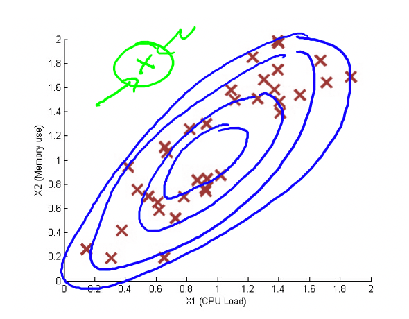
Voronoi Tesselation

When working with multidimensional data, plotting the nearest neighbor prediction results in a Voronoi tesselation, also known as a Voronoi diagram. This diagram divides the space into regions based on the closest data point for each query point.

Distance Metrics

Distance metrics play a crucial role in nearest neighbor algorithms. Some commonly used distance metrics include:

  • Euclidean distance: Measures the straight-line distance between two points in the feature space.
  • Scaled Euclidean distance: Allows for different weights on different dimensions, which is useful when certain features carry more importance. For example, in predicting house prices, the square footage may be weighted more heavily than the number of floors.
  • Other examples of distance metrics include Mahalanobis distance, rank-based distance, correlation-based distance, cosine similarity, Manhattan distance, and Hamming distance.

1 NN in Practice

The 1 NN algorithm performs well when the data is dense. However, there are limitations to its effectiveness:

  • In non-dense data regions, it struggles with interpolating between observations.
  • It is sensitive to noise, as a single noisy data point can significantly impact the prediction.
  • 1 NN tends to overfit the training data, resulting in poor generalization to new observations.

To address these limitations, the k-nearest neighbors (kNN) algorithm is often employed.


k-Nearest Neighbors (kNN)

In the kNN algorithm, we consider the k nearest neighbors and use their responses as predictions. This approach helps reduce the impact of noise compared to using only the nearest neighbor (1NN).

Challenges:

  1. Boundary issues: When dealing with boundaries, the same points may repeatedly appear as nearest neighbors, resulting in a flat response.
  2. Sparse region issues: In sparse regions, the same points may also be repeatedly chosen as neighbors, leading to potential inaccuracies.
  3. Discontinuity of fit: The fit obtained using kNN may not be smooth since one neighbor can suddenly be excluded from the set of nearest neighbors.

To address these challenges, we can employ weighted kNN, which assigns different weights to each neighbor based on their proximity.

Weighted k-Nearest Neighbors (kNN):

In weighted kNN, less weight is assigned to neighbors that are farther away from the query point. This approach helps mitigate the issue of fit discontinuity in standard kNN.

There are two common weighing schemes used in weighted kNN:

  1. Simple weighing scheme: In this scheme, the weight assigned to each neighbor is inversely proportional to its distance from the query point. The formula for weight calculation is: weight = 1 / distance.
  2. Sophisticated weighing scheme using kernels: Kernels, such as the Gaussian kernel, are employed to assign weights. The Gaussian kernel never reaches zero, ensuring that even distant neighbors have some influence. On the other hand, kernels like the Uniform or triangular kernel eventually reach zero, diminishing the influence of distant points. The parameter λ is used to control how quickly the kernel reaches zero. A faster decay indicates that distant points will have less influence.

By incorporating weighting schemes in kNN, we can achieve a more nuanced and smoother fit, addressing the issue of fit discontinuity encountered in standard kNN.

Kernel Regression:

Kernel regression is an alternative approach to kNN, where instead of considering only k neighbors, we consider all observations in the dataset. This allows for a more continuous and smoother prediction.

The choice of kernel in kernel regression can be either bounded, such as the uniform or triangular kernel. In such cases, we consider a subset of neighbors, but it is not strictly a kNN approach.

When performing kernel regression, two decisions need to be made:

  1. Choice of kernel: The choice of kernel has a relatively smaller impact on the prediction. Various kernels can be used, and their selection is typically based on the specific problem at hand.
  2. Choice of bandwidth: The bandwidth plays a more significant role in the prediction. It determines the spread of the kernel before it reaches zero. A small bandwidth can lead to overfitting, capturing noise and local fluctuations, while a large bandwidth can result in an overly smoothed fit, leading to high bias. The bandwidth can be tuned using the kernel’s parameter λ, which can be selected through techniques such as cross-validation.

By considering all observations and utilizing kernels in kernel regression, we can achieve a more flexible and continuous prediction model, providing a trade-off between bias and variance based on the choice of bandwidth.

Local Linear Regression

Up until now, we have discussed the use of weighted averages for prediction. However, an alternative approach is to fit a model in the vicinity of the prediction point, where the errors are weighted by a kernel.

In local linear regression, we can fit either a linear model or a quadratic model near the prediction point. A linear model is particularly useful for addressing boundary effects, as it provides a linear prediction instead of a constant one.

On the other hand, a quadratic fit can handle curvature in the data but may introduce higher variance in the predictions. Consequently, in practice, a linear fit is often recommended due to its favorable balance between bias and variance.

By employing local linear regression, we can adapt the model’s behavior based on the local data characteristics, enabling more accurate predictions near the prediction point.

Global vs Local Fit

In certain situations, we may find that a linear fit is appropriate for some regions of the input space, while a quadratic fit is more suitable for others. However, determining the breakpoints where the underlying structure changes can be challenging.

Non-parametric models come to the rescue in such cases. Instead of assuming a specific functional form, these models allow for more flexibility in capturing the underlying patterns.

One example of a global fit is taking the average as a constant prediction. This approach provides a simple representation of the data but assumes a uniform behavior across all observations.

On the other hand, kernel regression offers a way to achieve a local fit by applying different weights to each observation. Nearer observations receive higher weights, enabling the model to adapt to local variations in the data.

By leveraging non-parametric models like kernel regression, we can capture both global and local characteristics of the data, allowing for more accurate and adaptive predictions based on the proximity of observations.

Limitations of Non-parametric Approaches

While non-parametric approaches like kNN offer flexibility and adaptability, they do have certain limitations.

  1. Dimensionality: In higher dimensions, non-parametric models require an exponentially large number of observations to accurately capture the underlying patterns. As the number of dimensions increases, the data becomes more sparse, making it challenging to find sufficient neighboring points for accurate predictions.
  2. Data Availability: Non-parametric models heavily rely on the availability of a large amount of data. When the dataset is limited or scarce, it becomes difficult to leverage the full potential of non-parametric approaches.
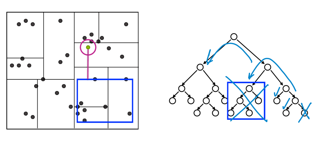
  3. Computational Complexity: Non-parametric models, such as kNN, involve a brute force search to find the nearest neighbors. This search operation has a complexity of O(N) for 1-NN and O(N log K) for k-NN, where N is the number of observations. While these complexities can be manageable for smaller datasets, they can become computationally expensive as the dataset grows larger.

To mitigate some of these limitations, techniques like clustering can be employed to reduce the search space and improve computational efficiency.

In situations where the dataset is limited or high-dimensional, parametric models offer an alternative by making certain assumptions about the underlying structure. These models provide a more compact representation and are often more suitable when data availability or computational complexity is a concern.

Understanding the limitations of non-parametric approaches helps in selecting the most appropriate modeling technique based on the specific characteristics of the dataset and the available resources.

References

Course by University of Washington

https://www.coursera.org/learn/ml-regression


On Clustering

K-mean is probably most popular algorithm and most taught algorithms in academia. However it has got many limitation and listing some of them here:

  • You need to specify value of k
  • Can cluster non-clustered data
  • Sensitive to scale
  • Even on perfect data sets, it can get stuck in a local minimum
  • Means are continuous
  • Hidden assumption: SSE is worth minimizing
  • K-means serves more as quantification


In Hierarchical clustering you don’t need to specify values of k, you can sample any level from the tree it build either by top down or bottom up approach. Such a tree is called Dendrogram.

Scikit also supports variety of clustering algorithms including DBSCAN and lists which one suits when. http://scikit-learn.org/stable/modules/clustering.html


References:

https://stats.stackexchange.com/questions/133656/how-to-understand-the-drawbacks-of-k-means