Step Size in Descent Methods

Descent Method

general_descent

  • When the descent direction is opposite to gradient is is called gradient descent.
  • We also have steepest descent and newton’s algorithm
  • In this post we will focus on line search
  • Term is called ‘line search’ because step size t determines where along the line {x + t ∇ x } next iterate will be. (ray search would be more appropriate term)


Fixed Step Size

  • Here we keep the step size (t) constant for all the iteration
  • Our solution many not converge if t is too large
  • If can take a lot of time if t is too small


faster_iteration


Exact line search

exact_line_search

  • It is used when cost of minimizing problem with one variable (s) is less than computing direction (∇ x)


Backtracking Line Search

  • Exact line search has to solve optimization problem and become computational inefficient
  • This is most widely used in practice.
  • Here we don’t find optimal value of t, but some approximation

inexact_line_searchonethreetwo


Demo of Convergence


faster_iteration


References


Simple Linear Program

Purpose is to know how it looks solving linear programs using libraries and solvers.

Reference : https://pythonhosted.org/PuLP/CaseStudies/a_blending_problem.html


\* Minimize food cost *\
Minimize
Total_Cost: 0.008 Beef_percentage + 0.013 chicken_percentag
Subject To
Fat_Constraint: 0.1 Beef_percentage + 0.08 chicken_percentag >= 6
Fiber_Constrint: 0.005 Beef_percentage + 0.001 chicken_percentag <= 2
Protine_Constraint: 0.2 Beef_percentage + 0.1 chicken_percentag >= 8
Salt_constraint: 0.005 Beef_percentage + 0.002 chicken_percentag <= 0.4
Total_Sum: Beef_percentage + chicken_percentag = 100
End


"""
THis is taken from https://pythonhosted.org/PuLP/CaseStudies/a_blending_problem.html
"""
from pulp import *
problem = LpProblem("Minimize food cost", LpMinimize)
x1 = LpVariable("chicken_percentag", lowBound=0)
x2 = LpVariable("Beef_percentage", lowBound=0, upBound=None)
problem += 0.013*x1 + 0.008*x2, "Total Cost"
problem += x1 + x2 == 100, "Total Sum"
problem += 0.1*x1 + 0.2*x2 >=8, "Protine Constraint"
problem += 0.08*x1 + 0.1*x2 >=6, "Fat Constraint"
problem += 0.001*x1 + 0.005*x2 <=2, "Fiber Constrint"
problem += 0.002*x1 + 0.005*x2 <=0.4, "Salt constraint"
problem.writeLP("minimize_food_cost.lp")
problem.solve()
print "Solution found was :", LpStatus[problem.status]
print "Here is the proportional of chick and beef that should be used"
for v in problem.variables():
print "\t",v.name, " : ", v.varValue
print "Cost will be : ", value(problem.objective)

view raw

pulp_LP.py

hosted with ❤ by GitHub


Solution found was : Optimal
Here is the proportional of chick and beef that should be used
Beef_percentage : 66.666667
chicken_percentag : 33.333333
Cost will be : 0.966666665

view raw

std_output.txt

hosted with ❤ by GitHub


Iterative Method for Unconstrained Optimization

There are two things

  1. Newton method for finding roots
    1. Does not have second order derivative in denominator
  2. Using 1 to solve for minima problem
    1. Minima problem is same as finding root of derivative  
    2. Has second order derivative in denominator
  3. There is a nice derivation starting from taylor series [3]

Newton’s Method

newton
  • Based on Taylor series expansion
  • Advantages
    • Convergence is rapid in general, quadratic near optimal point
    • Insensitive to no of variables
    • Performance does not depend on choice of parameter
      • Gradient method depends on learning rate
  • Disadvantages
    • Cost of computing and storing Hessian
    • Cost of computing single newton step
      • You need double derivative (Example in note is a simple root finding problem)

Gradient Descent

  • Very popular method and does not need any write up
  • Exhibits approximately linear convergence
  • Advantage
    • Very simple to implement
  • Disadvantage
    • Convergence rate depends on number of the Hessian
    • Very slow when for large no of variables (say 1000 or more)
    • Performance depends on choice of parameters like learning rate


Gradient Descent vs Netwon’s Method

Edit 1 : I believe term step is more suitable here. Gradient step and Newton step. Method is more suitable for interior point methods, active set methods, cutting plane methods and proximal methods.

Newton’s method for finding roots:

3

In optimization we are essentially finding roots of derivative.

1
2

We are approximating function using Taylor series. We are finding minimum of this approximated function. This root will be our new guess. This perspective is used in derivation.

4

Andrew N.G Lecture [2]

 Gradient Descent Newton
 Simpler Slightly more complex (Requires computing and inverting hessian)
 Needs choice of learning rate alpha No parameters (third point in image is optional )
 Needs more iteration Needs fewer iteration
 Each iteration is cheaper O(n) where n is no of features Each iteration is costly. Hessian is (n+1) * (n+1). Inverting matrix is roughly O(n^3)
 Use when no of features are less (n<1000) Use when (n > 10,000)

Gradient can only give you direction. If you want to know next point (or step size), second order derivative (hessian) is must.

Golden Section Search

  • Typically applicable for one dimension only
  • We used it to calculate mobile/tablet adjustments
    • As a good practice we had avoided recursion and took at max 20 iteration breaking loop with some criterion
  • Applicable for strictly unimodal function
  • Three points that maintain golden ratio (phi)
  • Following two problems are different :
    • Searching in rotated sorted array
    • Finding a max on uni-modal function
    • Formal has a property that left one end will be smaller than other, which later does not have
      • This property is used in binary search
  • What is special about golden ration ?
from math import sqrt
phi = (1 + sqrt(5))/2
resphi = 2 – phi
# a and b are the current bounds; the minimum is between them.
# c is the center pointer pushed slightly left towards a
def goldenSectionSearch(f, a, c, b, absolutePrecision):
if abs(a – b) < absolutePrecision:
return (a + b)/2
# Create a new possible center, in the area between c and b, pushed against c
d = c + resphi*(b – c)
if f(d) < f(c):
return goldenSectionSearch(f, c, d, b, absolutePrecision)
else:
return goldenSectionSearch(f, d, c, a, absolutePrecision)
f = lambda x: x**2
def test_search():
assert abs(goldenSectionSearch(f, -1, (-1 + resphi*2), 1, 1e-10)) < 1e-10
print "OK!"
if __name__ == '__main__':
test_search()

Reference

[0] http://www.ece.mcmaster.ca/~xwu/part4.pdf

*[1] https://www.youtube.com/watch?v=42zJ5xrdOqo

*[2] https://www.youtube.com/watch?v=iwO0JPt59YQ

[3] https://suzyahyah.github.io/calculus/optimization/2018/04/06/Taylor-Series-Newtons-Method.html

Quadratic Programming CVXOPT

This is taken from https://courses.csail.mit.edu/6.867/wiki/images/a/a7/Qp-cvxopt.pdf

General algorithms for QP (from wikipedia)


Standard form

qp1

Converting to standard form

qp2

Python Code


Loading

Sorry, something went wrong. Reload?
Sorry, we cannot display this file.
Sorry, this file is invalid so it cannot be displayed.

view raw

QP_CVXOPT.ipynb

hosted with ❤ by GitHub


[Example] Lagrange Multiplier With Equality Constraints


Stationary Point

Definition of stationary point from wikipedia :

In mathematics, particularly in calculus, a stationary point or critical point of a differentiable function of one variable is a point on the graph of the function where the function’s derivative is zero. Informally, it is a point where the function “stops” increasing or decreasing (hence the name).


Lagrange multiplier helps us to find all the stationary points, It can be local minima, local maxima, global minima or global maxima. Once we evaluate objective function at each of these stationary point we can classify which one is local/global minima and maxima.


Example


Lagrange Duality

There are three things :

  1. Original problem (Primal problem)
  2. Dual function (Function of lagrange multiplier)
  3. Dual problem


Suppose p is the solution of primal problem and d the dual problem.


If original problem is minimization, we are interested in lower bound (d) such that d<p.  We want to find maximum value of d and dual problem becomes maximization problem.


If original problem is maximization, we are interested in finding upper bound (d) such that p<d. We want to find minimum value of d and dual problem become minimization problem.


Dual problem is always convex irrespective of primal problem.


d<p is weak duality, while d=p is strong duality.

If primal problem is convex strong duality generally holds.

Slater’s condition is sufficient tests for convex optimization.


Further reading :

Kanpsack Problem here 

Click to access classbfs121109082344836.pdf

Convex Optimization by Stephen Boyd


[Theory] Lagrange Multiplier and Constrained Optimization

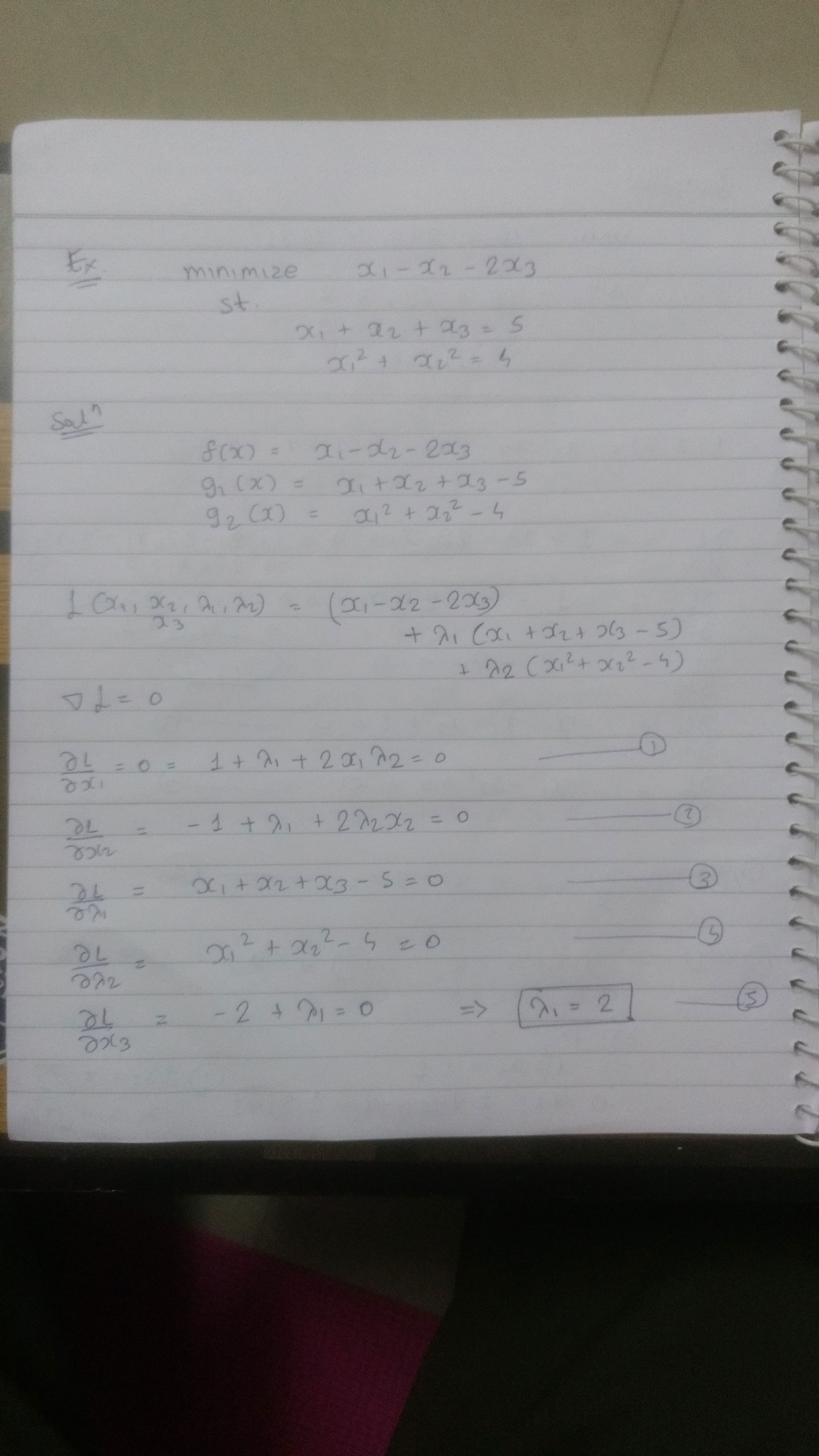
Lagrange multipliers helps us to solve constrained optimization problem.

An example would to maximize f(x, y) with the constraint of g(x, y) = 0.

Geometrical intuition is that points on g where f either maximizes or minimizes would be will have a parallel gradient of f and g

∇ f(x, y)  =  λ ∇  g(x, y)

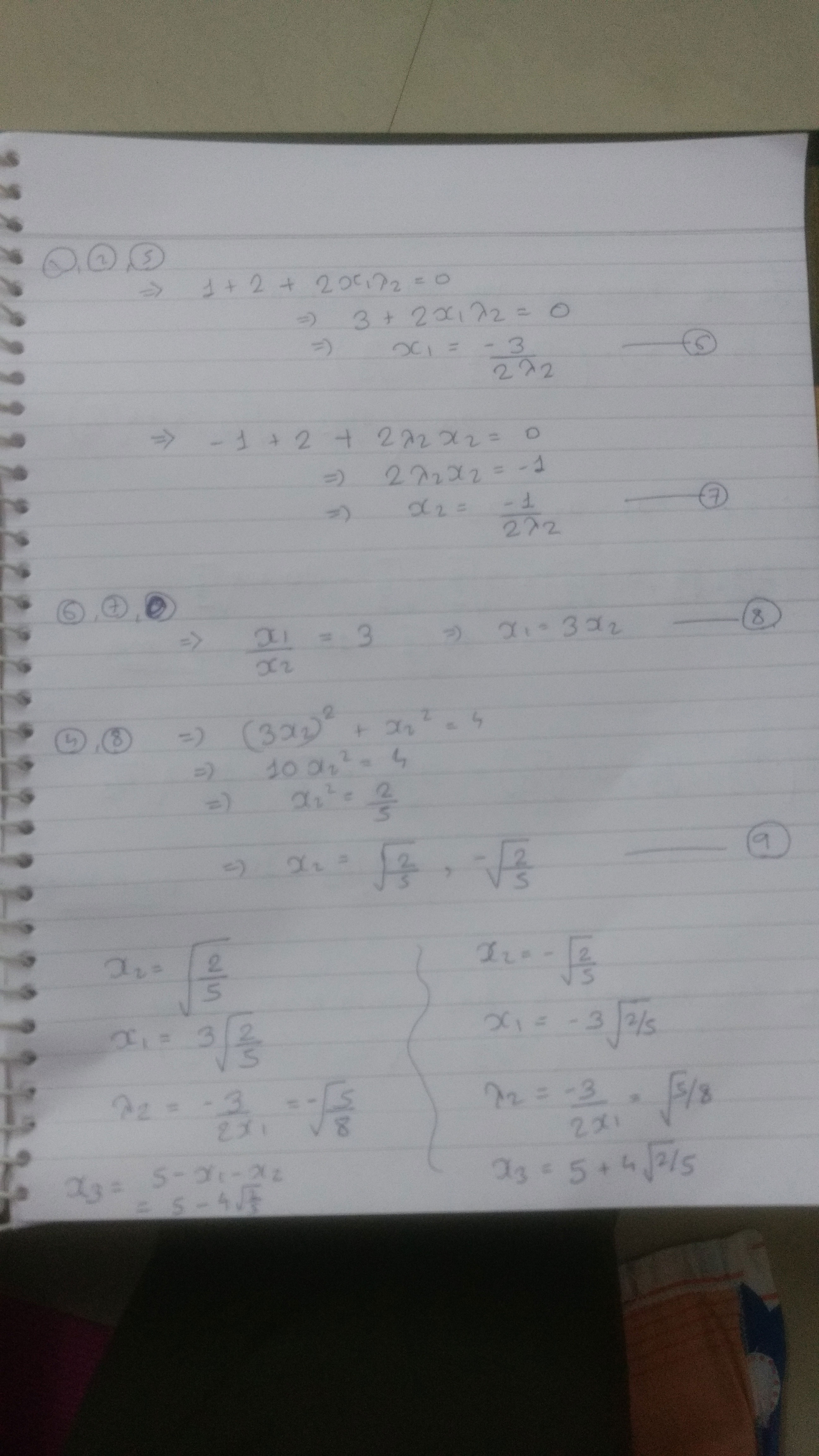
We need three equations to solve for x, y and λ.

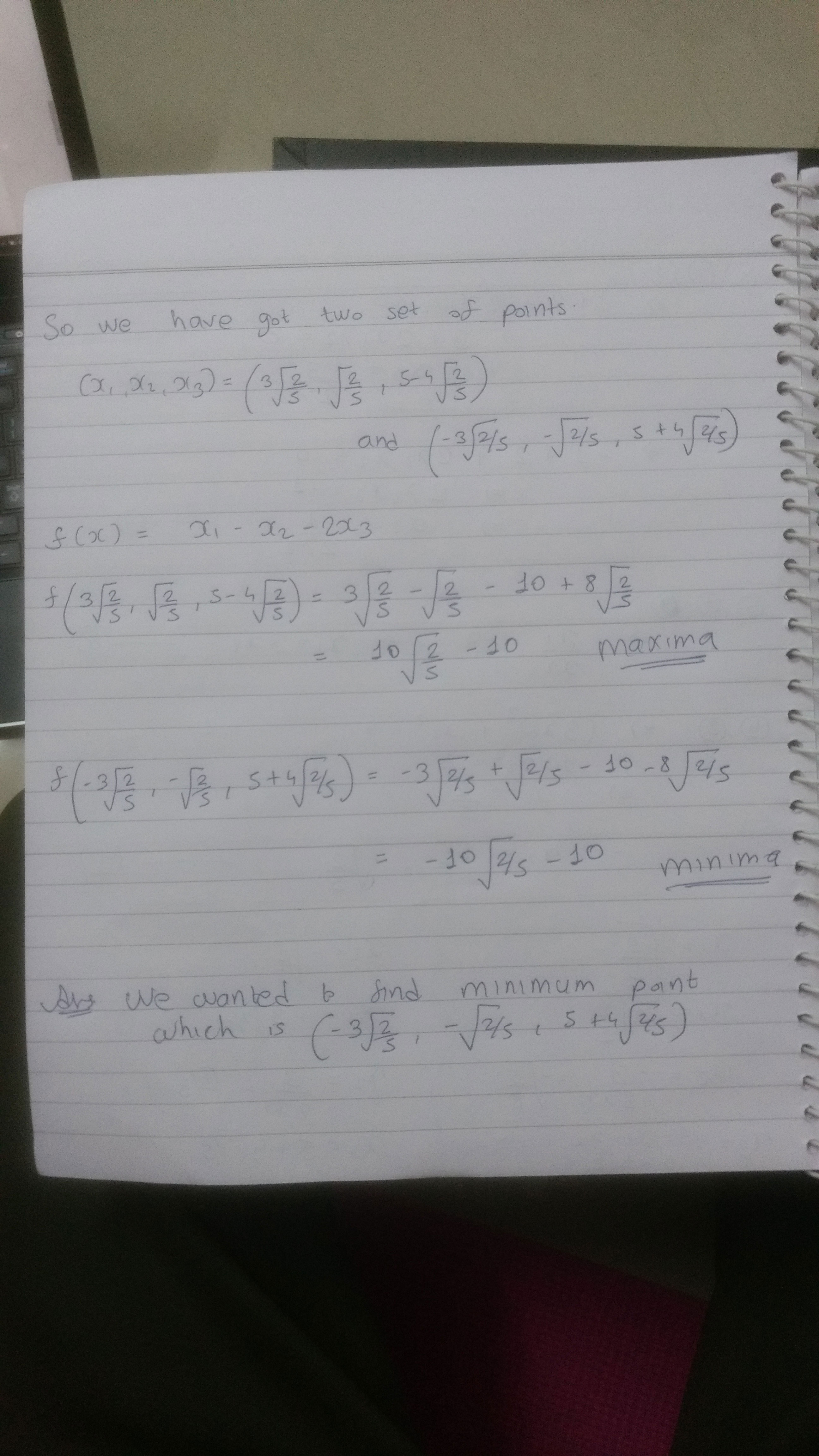
Solving above gradient with respect to x and y gives two equation and third is g(x, y) = 0

These will give us the point where f is either maximum or minimum and then we can calculate f manually to find out point of interest.

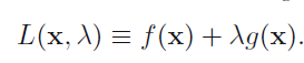
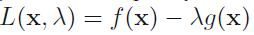
Lagrange is a function to wrap above in single equation.

L(x, y, λ) = f(x, y) – λ g(x, y)

And then we solve ∇ L(x, y, λ) = 0


Budget Intuition

Let f represent the revenue R and g represent cost C.

Also let g(x, y) = b where b is maximum cost that we can afford.

Let M* be the optimized value obtained by solving lagrangian and value of λ we got was λ*.

l1

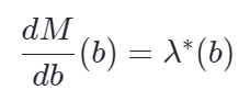
So λ is the rate with which maximum revenue will increase with unit change in b.


Inequality Constraint


Here is the problem of finding maximum of f(x) [2]

l5

l4l7

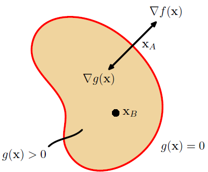
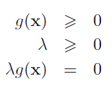
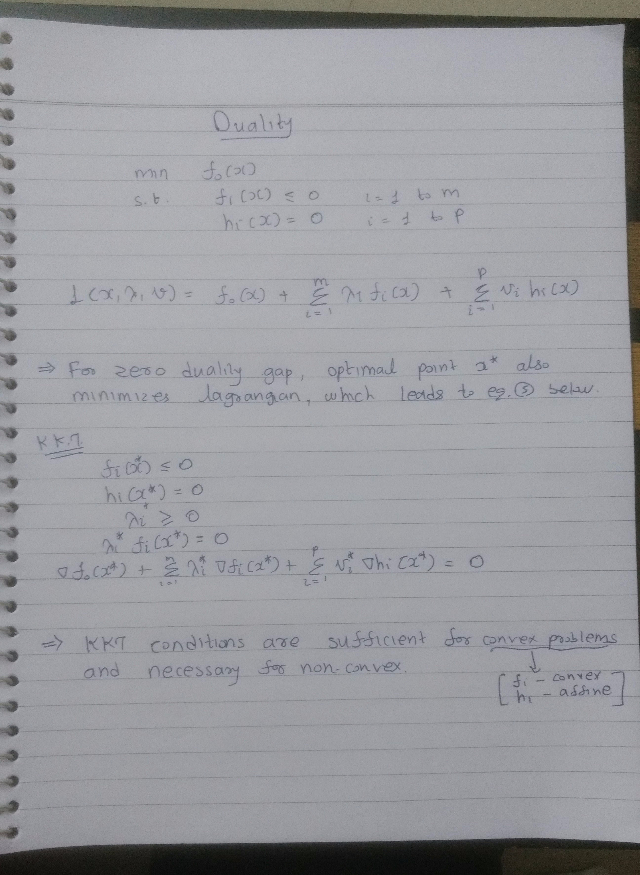
Above conditions are known as Karush-Kuhn-Tucker (KKT) conditions.

First – primal feasibility

Second – dual feasibility

Third  –  complementary slackness conditions

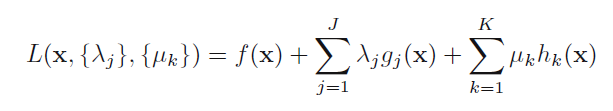
For the problem of finding minimum value of f(x) we minimize following with same KKT conditions:

l9


This can be extended to arbitrary number of constraints.

l8


Notes

  • This is relates to solving the dual of a problem for convex function as we had in Boyd’s book
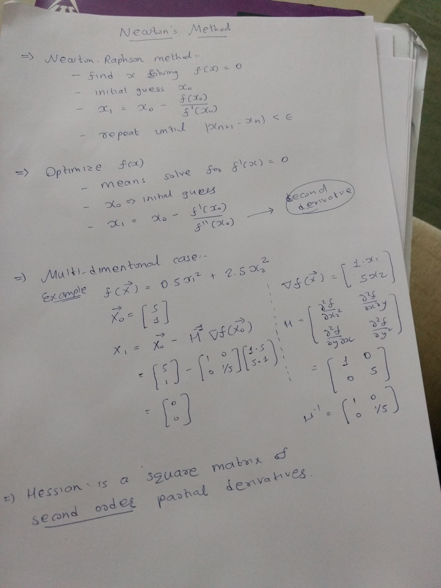
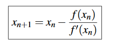
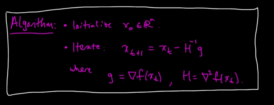
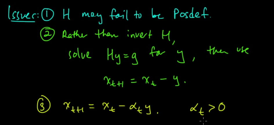
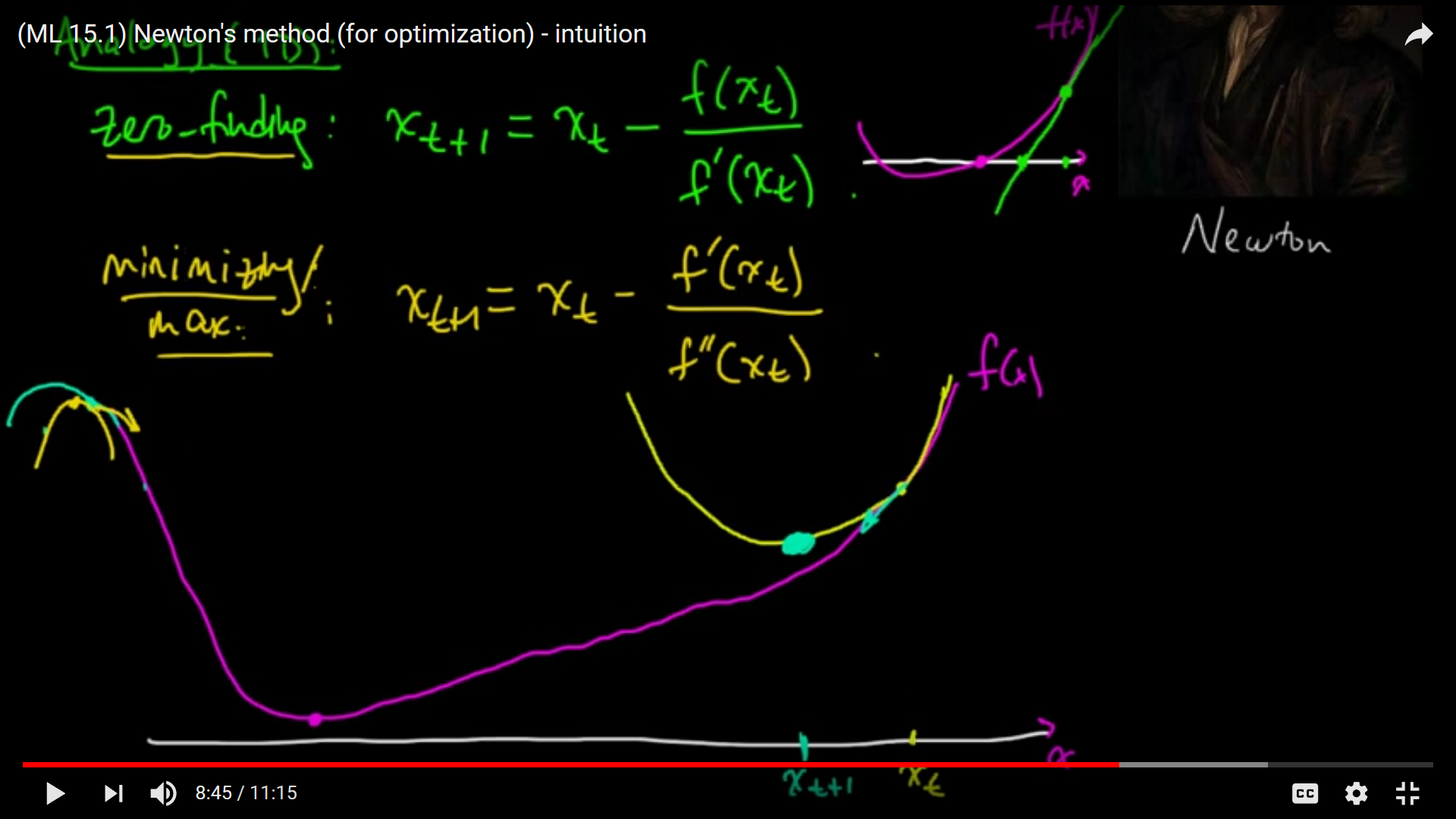
  • For unconstrained optimization computing hessian of a matrix is one way of solving if it is continuous  [1]


formal summary

References

[0] https://www.khanacademy.org/math/multivariable-calculus/applications-of-multivariable-derivatives/constrained-optimization/a/lagrange-multipliers-single-constraint

[1] https://www.youtube.com/watch?v=TyfZaZSF5nA

[2] Pattern Recognition and machine learning by Bishop