What does CLT says ?
- Sum of random samples forms normal distribution
- This samples may not come from normal distribution
- Sum forming random distribution implies that mean would also form normal distribution
Straight facts
- Central limit theorem helps getting confidence interval for parameters
- It works for all distributions when n > 30
- For normal distribution it works even if n < 30
- Why do we need to have distribution
- To make variance estimation stable
- We want to have just one unknown that is mean
- We need to test normality of samples before applying t-test
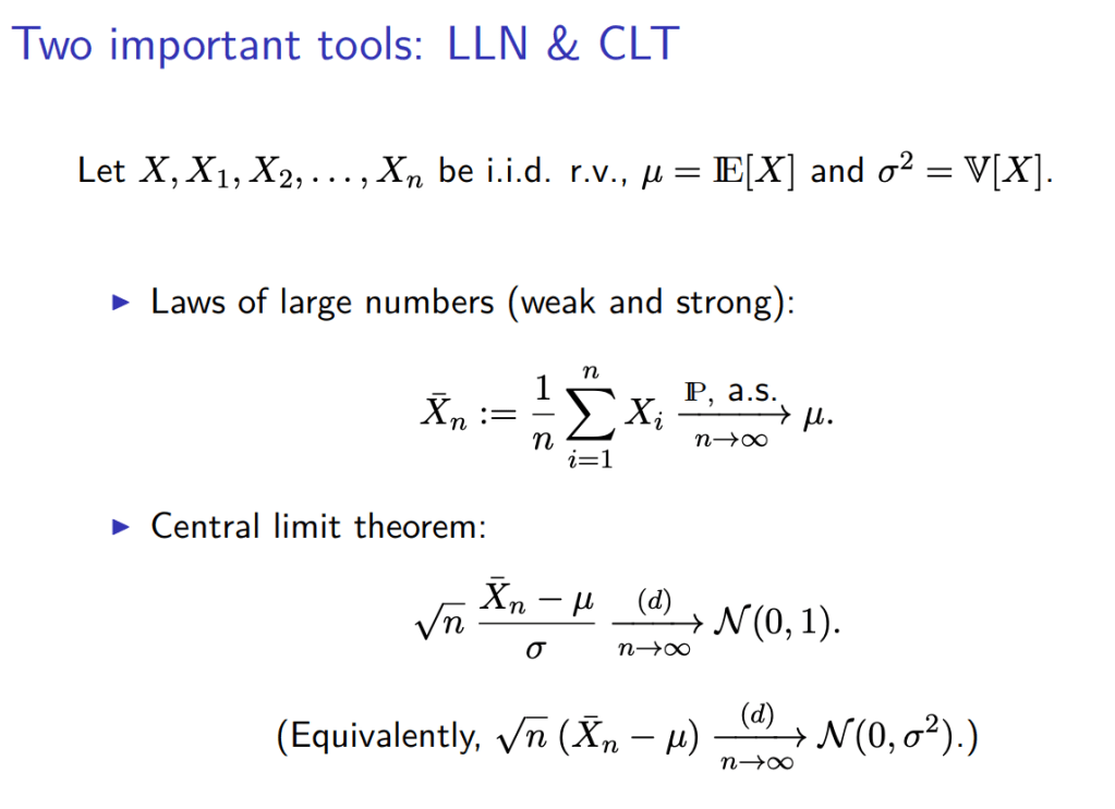
Slide from MIT course : https://ocw.mit.edu/courses/mathematics/18-650-statistics-for-applications-fall-2016/
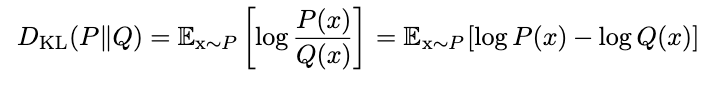
sigma / (sqrt(n)) is standard error of mean. We are saying this distribution reaches to standard normal distribution.
Law of Larger Number
- As a sample size grows, its mean gets closer to the average of the whole population. This is due to the sample being more representative of the population
Example:
- During significance testing we calculate left hand side. For examples testing fairness of coin that number comes out to be 3.54. Now for standard normal 3*sigma = 3*1 = 3 is 99 % of area. We are further away than it. So we can reject null hypothesis. [1]
- Thing to understand is that distribution of Bernoulli parameter(p) is normal.
- We are not saying how far observed mean is from 0.5 in Bernoulli distribution. If we were doing that we would not have used sqrt(n).
- Also more importantly Bernoulli can take only two values 0 and 1. From that perspective as well it does not make sense.
- See the equation in the slide below in central limit theorem. It is a normal distribution N(0,1).
Refereces
[0] : Slide from MIT course : https://ocw.mit.edu/courses/mathematics/18-650-statistics-for-applications-fall-2016/