Support Vector Machines

Maximum margin classifiers

Also known as optimal separating hyperplane
Margin is the distance between hyperplane and closest training data point
We want to select a hyperplane for which this distance is maximum
Once we identify optimal separating hyper plane there can be many equidistance training points with the shortest distance from hyperplane
Such point are called support vectors
- These points support the hyperplane in a sense that if they are moved slightly optimal hyperplane will also move

Training

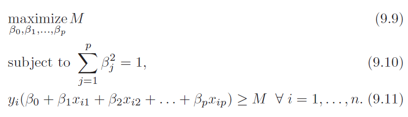
Equation 9.10 ensures that left hand side of equation 9.11 gives perpendicular distance from the hyperplane
Equation assumes y has two values (+1) and (-1)

Maximum margin classifier does not work when supporting hyperplane does not exist.
Support vector classifier relaxes optimization objective to get that work
Unlike maximum margin classifier this one is less prone to overfit as well
- The formal one is very sensitive to change in single observation
Also know as soft margin classifier

ε variable allows training point to be on wrong side of margin
- If ε > 0 it is on the wrong side of margin
- If ε > 1 it is on the wrong side of hyperplane
Parameter C is the budget that constraints how many points are allowed on wrong side of hyperplane
C is selected with cross validation and controls bias variance trade off
Point that lies directly on the margin or on the wrong side of margin for their class are called support vectors
- Because these points affects the choice of hyperplane
- And this is the property which makes it robust to outliers
  - LDA calculates mean of all the observation
  - However LR is less sensitivity to outliers
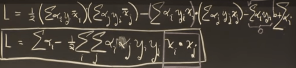
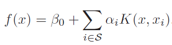
Computation note – when we try to solve above optimization problem with lagrange multiplier we found that it depends on dot product of training samples
- This will be very important when we discuss support vector machine in next section
- Dot product is only with support vector, both while training and while solving [1]

One solution is to create polynomial features (as we generally do for LR)
But fundamental problem with this approach is that how many and which terms you should create
Also creating large number of feature raises computational problem

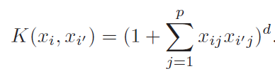
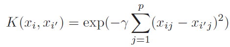
For the case of SVM, that fact that it involved only dot product of observation allows us to perform kernel trick.
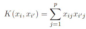
Kernel acts as similarity function
Above equation makes it clear that we are not calculating(and storing) higher order polynomial still taking the advantage of it
Second one is polynomial kernel and last one is radial kernel
This video shows visualization of kernel trick

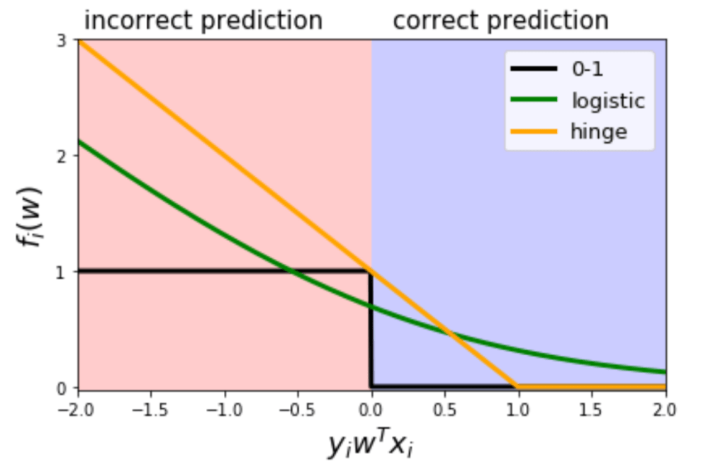
Loss is 0 for w*x which are not support vectors
Look at equation 9.14 and 9.15 above
- Looking at its property episilon, it relates to hinge loss
- Yet to check it in SVM lagrange solution though
In hinge loss also we would predict +1 if w*x > 0 else -1
Why not keep boundary at 0
- This can make w a zero to make positive training example right
- Zero parameter vector would mean while prediction we would always get 0
  - Because prediction is w*x
  - This makes it difficult to assign labels during prediction
- We keep boundary away from 0 to make zero we don’t get 0 parameter vector

[0] : An Introduction to Statistical Learning – http://www-bcf.usc.edu/~gareth/ISL/