In standard linear regression we make two assumption :

1. P(Y/X) is a normal distribution
2. Mean is a linear function of parameter µ  = β*X
3. P(Y/X) = Ν(µ, σ^2* I)       # σ is standard deviation and I is identity matrix

In GLM we relax two things :

1. P(Y/X) is from any exponential family
2. Mean is some function of β*X
   1. µ = f(β*X)
   2. g(µ) = β*X
   3. g = f^(-1)
   4. g is called link function

Example of link functions:

1. log link
2. reciprocal link
3. logistic link

Derivation of log-likelihood matches that of normal distribution. However closed form solution is not defined and is generally solved by least square and convex optimization.

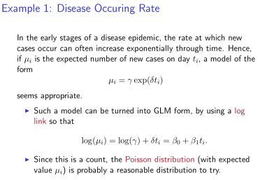
Here is one example from MIT course mentioned in references.

Logistic

• In gaussian regression we predict μ for each sample
  • This μ comes from β0, β1, β2 which are same for each sample
• For binomial regression we want to predict p for each sample
  • This p comes from β0, β1, β2 which are same for each sample
• One option :
  • p = β0 + β1*x1 + β2*x2
• Second option
  • p = sigmoid (β0 + β1*x1 + β2*x2)
  • f(p) = log(p/(1-p)) = β0 + β1*x1 + β2*x2
  • It is logit link function
• What are other options apart from sigmoid
  • step function (Not differentiable, that is why we use (sigmoid)
  • tanh is sometime used in deep learning
• What if we go with option 1:
  • Binomial distribution requires p to be in (0,1)
• Example :
  • How many fishes survive (alive/dead) given food and water

Poisson

• Poisson distribution models probability of observing count
  
  
  
  • 
    
    
    
    • P(k) = exp(-λ) * (λ^k) / k !
    
    
    
    
  
  
  
  

  Parameter λ >= 0

• Option one:
  • λ = β0 + β1*x1 + β2*x2
• Option two:
  • λ = exp ( β0 + β1*x1 + β2*x2 )
  • f ( λ ) = log ( λ ) = ( β0 + β1*x1 + β2*x2 )
  • It is log link function
• What if we go with option one:
  • We want λ > 0
  • Relationship between input and output is not additive but multiplicative ?
    • Suppose the seeds have germinated as many as 1.5 times by the enough water and as many as 1.2 times by the enough fertilizer. When you give both enough water and enough fertilizer, the seeds would germinate as many as 1.5 + 1.2 = 2.7 times ?
      
      Of course, it’s not. The estimated value would be 1.5 * 1.2 = 1.8 times. [3]
• Example:
  • How many seed will germinate given water and fertilizer

Parameter Estimation

• We can do maximum likelihood estimate and find parameters β0, β1, β2
• Deriving maximum likelihood for binomial:
  • max_lh = Multiply (Likelihood of y_acutal of each sample for predicted distribution)
  • max_lh = Multiply ( Binomial(p) )
  • max_lh = Multiply ( p if y=1 else (1-p) )
  • log(max_lh) = Summation (y*logp + (1-y) log (1-p))
• Deriving maximum likelihood for Poisson:
  • max_lh = Multiply (Likelihood of y_acutal of each sample for predicted distribution)
  • max_lh = Multiply ( Poisson (u) )
  • max_lh = Multiply (exp(-u) * u^y / y! )
  • log(max_lh) = summation ( -u + y*log(u) – log (y!) )
• Above two are rough derivations but conveys the idea
• For Gaussian it turns out to OLS (Ordinary Least Squares) and has closed form solution
• For other we solve it via gradient/newton’s method.

Why the gradient is the same for linear and logistic regression

If you write gradient descent for linear regression and then for logistic regression, you end up typing the same line twice:

grad = X.T @ (y_pred - y) / n

That is not a coincidence or a happy accident of notation. It is a theorem, and it explains a design decision that shows up throughout deep learning.

The pattern

Identical in every case: X^T × (prediction − target).

Why: the cancellation

Apply the chain rule to logistic regression and watch what happens. With z = Xw and p = σ(z):

∂L/∂w = (∂L/∂p) · (∂p/∂z) · (∂z/∂w)

The two middle terms are:

∂L/∂p = (p − y) / [p(1 − p)]      ∂p/∂z = p(1 − p)

The p(1 − p) cancels exactly. What survives is (p − y) · X, and the transpose assembles it into X^T(p − y).

For linear regression there is nothing to cancel. The link is the identity, so ∂ŷ/∂z = 1 and you get the same form trivially.

The general statement

This is the canonical link property of generalized linear models. For any exponential-family likelihood

p(y | θ) = h(y) · exp( θy − A(θ) )

the mean is μ = A′(θ) and the variance is A″(θ). When you use the canonical link — meaning you set θ = Xw directly — the score function is always

∇_w ℓ = X^T(y − μ)

The curvature term A″ that the chain rule produces is exactly the same A″ sitting in the denominator of the loss derivative. It cancels by construction, because the link and the loss are both derived from the same log-partition function A(θ).

• Linear → Gaussian, A(θ) = θ²/2, identity link
• Logistic → Bernoulli, A(θ) = log(1 + e^θ), logit link
• Poisson → A(θ) = e^θ, log link

One object, three instances.

Where it breaks, and why that matters

Pair a sigmoid with MSE instead of log-loss and the cancellation fails:

∇_w = X^T [ (p − y) · p(1 − p) ]

The extra p(1 − p) survives, and it is near zero whenever p is near 0 or 1. Measured on a small synthetic dataset at a weight vector where many predictions are confidently wrong:

log-loss gradient norm:  0.770
MSE      gradient norm:  0.014

Fifty-five times smaller, in exactly the regime where the largest correction is needed. The model is badly wrong and the gradient says “barely move.”

That is the vanishing gradient problem in its simplest form, and it is why cross-entropy replaced squared error for classification. MSE paired with a sigmoid is also non-convex in w, so it has local minima; log-loss is convex.

It still converges on easy data — 200,000 iterations reached a negative log-likelihood of 0.3100 against log-loss’s 0.3098 in 1,000 — but that is roughly 200 times slower on a trivial problem. On anything harder it simply stalls.

The short version

The gradient is X^T(prediction − target) for any GLM paired with its canonical link, because the link’s derivative cancels the loss derivative — both come from the same log-partition function. That is not a convenience. It is the reason those particular loss and activation pairs became the standard ones.

References :

[0] https://ocw.mit.edu/courses/mathematics/18-650-statistics-for-applications-fall-2016/lecture-slides/MIT18_650F16_GLM.pdf

[1] Wonderful MIT lecture : https://www.youtube.com/watch?v=X-ix97pw0xY

[2] https://onlinecourses.science.psu.edu/stat504/node/216/

[3] https://tsmatz.wordpress.com/2017/08/30/glm-regression-logistic-poisson-gaussian-gamma-tutorial-with-r/