Thompson sampling is one approach for Multi Armed Bandits problem and about the Exploration-Exploitation dilemma faced in reinforcement learning. It is also know as posterior sampling.

Challenge in solving such a problem is that we might end up fetching the same arm again and again. Bayesian approach helps us solving this dilemma by setting prior with somewhat high variance.

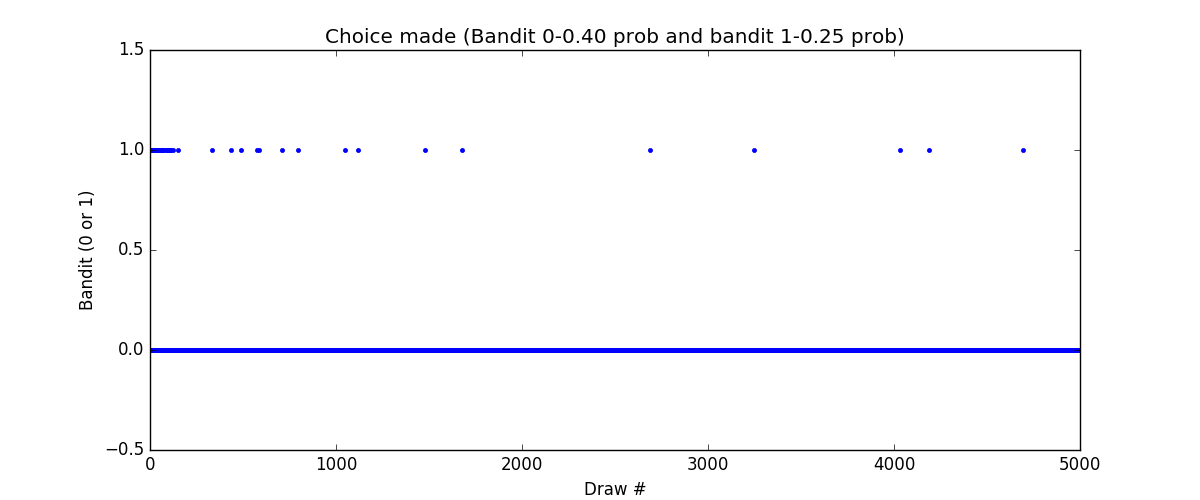
Here is the code for two armed bandit. One has success probability of 40% (bandit 0) and another has 25% (bandit 1).

We are using beta distribution for deciding which arm to pull. Beta distribution has two parameter alpha and beta. Higher values of alpha, pulls distribution towards 1. Beta distribution is always confined between 0 and 1.

How we train is that for each feedback we receive we increment alpha by 1 if it was success or beta by 1 in case of failure. For choosing the arm we draw random sample from the distribution of each arm and select the arm with highest value.

	import numpy as np
	import scipy.stats as stats
	from matplotlib import pyplot as plt
	class BetaThompson:
	def __init__(self, num_bandits, prior_a, prior_b):
	self.num_bandits = num_bandits
	self.a = prior_a
	self.b = prior_b
	def learn(self, bandit, success):
	if success:
	self.a[bandit]+=1
	else:
	self.b[bandit]+=1
	def suggest(self):
	sampled_prob = []
	for i in range(self.num_bandits):
	dist = stats.beta(self.a[i], self.b[i])
	prob=dist.rvs()
	sampled_prob+=[prob]
	return sampled_prob.index(max(sampled_prob))
	class Gamble:
	def __init__(self, num_bandits, binom_mean):
	self.num_bandits=num_bandits
	self.binom_mean=binom_mean
	def gamble(self, bandit_no):
	dist=stats.binom(n=1,p=self.binom_mean[bandit_no])
	success = True if dist.rvs()>0.5 else False
	return success
	def main():
	g = Gamble(2, [0.40, 0.25])
	bot = BetaThompson(2, [1,1], [1,1])
	choice=[]
	for i in range(5000):
	suggestion = bot.suggest()
	result = g.gamble(suggestion)
	bot.learn(suggestion, result)
	choice+=[suggestion]
	plt.figure(figsize=(12,5))
	plt.plot(choice, 'b.')
	plt.ylim([-0.5,1.5])
	plt.title('Choice made (Bandit 0-0.40 prob and bandit 1-0.25 prob)')
	plt.xlabel('Draw #')
	plt.ylabel('Bandit (0 or 1)')
	plt.savefig('choice.png')
	if __name__== "__main__":
	main()

view raw thompson_sampling.py hosted with ❤ by GitHub

And here is simulation results. We see that initially both the the armed are pulled frequently but slowly arm 1 is pulled less and less, but it is never straight away zero.

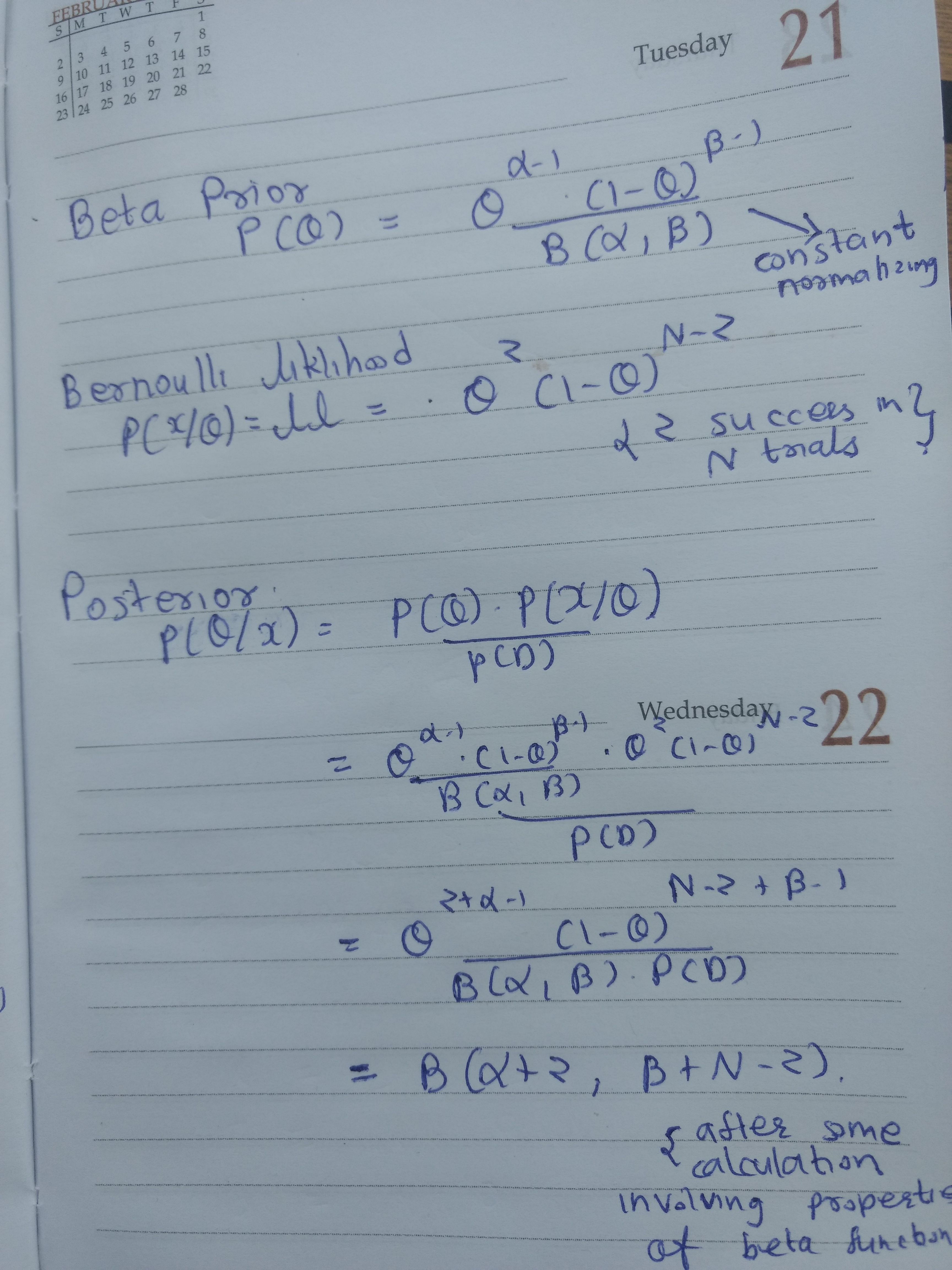
Math Behind Increasing alpha and beta

In one line posterior is beta distribution for beta prior and Bernoulli likelihood. In other words beta is a conjugate prior for Bernoulli likelihood. List of various conjugate prior is available at [1].

PDF of beta distribution is simple once you think in terms of the effect of alpha and beta.

Look at note below, formula of beta distribution is not complex, actually it is very similar to

References

[1] : https://ocw.mit.edu/courses/mathematics/18-05-introduction-to-probability-and-statistics-spring-2014/readings/MIT18_05S14_Reading15a.pdf