Edit : Extended post is available here

Some Scenarios

• In finance default is failure to meet the legal obligation of loan. Given some data we want to classify whether the person will be defaulter or not.
  • Suppose our training data-set is imbalanced. Out of 10k samples only 300 are defaulters. (3%)
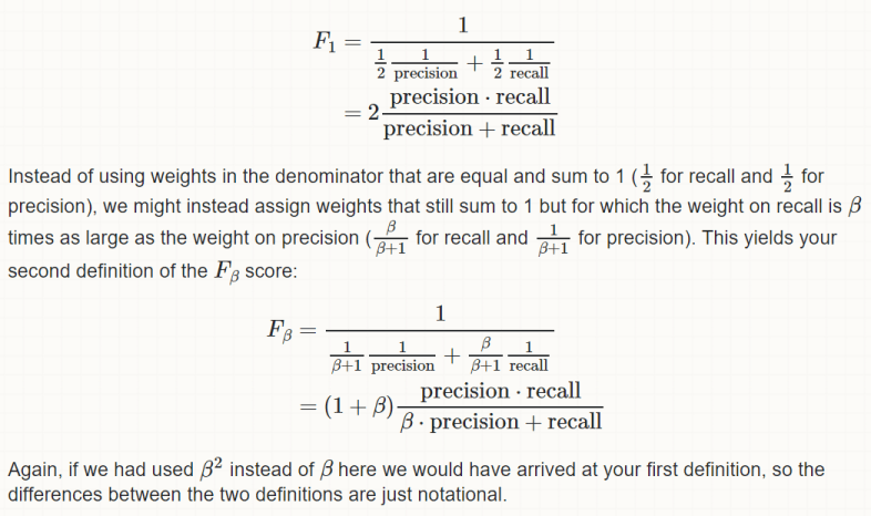
  • Classifier in the following table is good at classifying non defaulters but not good at classifying defaulters (which is more important for credit card company)
  • Assume what if out of 300 defaulters 250 are classified as non defaulters and given the credit card
• Doctors want to conduct a test whether a patient has cancer or not.
  • Popular terms in medical field are sensitivity and specificity
  • Instead of trying to classify person as defaulter, here we classify if patient has cancer.
  • Sensitivity = 81/333 = 24 %
  • Specificity = 9644/9667 = 99 %
  • Every medical test thrives to achieve 100% in both sensitivity and specificity.
• In information retriever we want to know how many % of relevant pages we were able to retrieve.
  • TP = 81
  • FP = 23
  • TN = 9644
  • FN = 252
  • Precision = 81/104= 77%
  • Recall = 81/333= sensitivity = 24%

Example

• Formulas:
  • Precision = TP/(TP+FP)
  • Recall = TP/(TP+FN)
  • Sensitivity = TP/(TP+FN)
  • Specificity = TN/(TN+FP)
  • Recall and sensitivity are same

Solution is to change the threshold

• Earlier we were assigning person to default if probability is more than 50%
• Now we want to assign more person as defaulter
• So we will assign them to defaulter when probability is more than 20%
• This will incorrectly classify non-defaulters to defaulters but that is less concerned compared to assigning defaulter to non-defaulter
  • This will also increase the overall error rate, which is still okay

ROC-AUC

• We can always increase sensitivity by classifying all samples as positive
• We can increase specificity by classifying all samples as negative
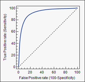
• ROC plot (sensitivity) vs (1-specificity)
  • That is TP vs FP
  • And also precision vs recall
• ROC = Receiver operating characteristic
• It is good to have ROC curve on top left
  • Better classifier
  • Accurate test
• And ROC curve close to 45 degree represents less accurate test
• AUC = Area Under Curve
  • Area under ROC curve
• Ideal value for AUC is 1
• AUC of 0.5 (45 degree line) represents a random classifier
• AUC = P(score of a random positive > score of a random negative )
  • 0.5 => random, 1 => perfect seperation
  • Its scale invariance
    • Any monotonic transform ( multiply by 1.4, log ) preserves parities comparison

How to plot ROC?

• Change the probability threshold from 0 to 1 and measure sensitivity and specificity. If specificity keeps on decreasing ((100-specificity) keeps on increasing) as sensitivity increase it is a bad classifier.
• For random classifier ROC is 45 degree line
  • You draw random number between (0, 1)
  • Classify it based on threshold
  • So threshold is there
  • But while building classifier we want to do better than drawing random probability between (0, 1). We also want to consider features into account while drawing between (0, 1)
• Can AUC be less than 0.5? I don’t think so.
  • Complementing the output will bring it to other side of line anyway.
• What if I classified all of them as positive?
  • That means you are taking all 1. You can not plot ROC with that.

Threshold selection

• Unless there is special business requirement (as in credit card defaulters) we want to select a threshold which maximizes TP while minimizing FP
• There are two methods to do that:
  • Point which is closest to (0, 1) in ROC curve
  • Youden Index
    • Point which maximizes vertical distance from line of equality (45 degree line)
    • We can derive that this is the point which maximizes (sensitivity + specificity)

AUC vs overall accuracy as comparison metric

• AUC helps us understand how much our classifier is away from random guess, which accuracy can not tell
• Accuracy is measured at particular threshold while AUC requires moving threshold from 0 to 1

PR-AUC

PR-AUC (Precision-Recall Area Under the Curve) summarizes a classifier’s performance by plotting Precision against Recall across all thresholds. You should use it when your data has a severe class imbalance (e.g., < 5% positive class) and your primary goal is to minimize False Positives and False Negatives within that rare target group

• While training on the model, you can take a look at PR-ROC. Once you have found your best model, you can pick up any point based on the business needs.
• A random classifier always gives ROC AUC to be 0.5.
  • Our ROC would be the percentage of positive samples.
  • This helps with the cases where there is highly class imbalance and we have more negative samples.

F score

• We know that recall and sensitivity are same, but precision and specificity are not same
• While medical field is more concerned about specificity, information retrieval is more concerned about precision
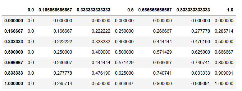
• So they came up with F score which is harmonic mean of precision and recall
• AUC helps us maximizing sensitivity and specificity simultaneously while F score helps us maximizing precision and recall simultaneously
• Beta in f score helps providing weight to precision and recall.
• Harmonic mean can not be made arbitrarily large while changing some values to bigger one and leaving at least one unchanged. It is maximizes when all elements are increased.
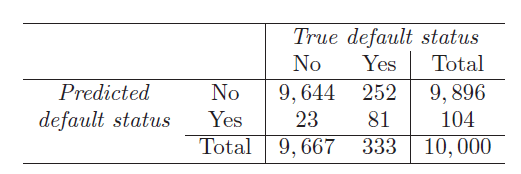
  • x = 0, y = 1 will give 0.5 in arithmetic mean but is zero for harmonic mean

Micro and Macro F1 Score

The Core Difference

When dealing with multi-class classification (predicting three or more categories, like Cat, Dog, or Bird), you calculate an F1-score for each individual class. To get a single final score for the whole model, you must aggregate them:

• Macro F1 treats all classes equally. It calculates the F1-score for each class independently and takes the unweighted average. It is excellent for flagging if a model performs poorly on a rare, minor class.
• Micro F1 treats all samples equally. It pools the True Positives (TP), False Positives (FP), and False Negatives (FN) from all classes together, then computes a global F1-score. It is heavily influenced by the performance of the majority class.

Step-by-Step Example

Let’s say we have an image classification model evaluating 100 test images across three categories. The dataset is highly imbalanced:

• Cat: 80 images
• Dog: 15 images
• Bird: 5 images

After running our model, we track the True Positives (TP), False Positives (FP), and False Negatives (FN) for each class:

(Note: Our model does great on Cats, decent on Dogs, but terrible on Birds because Birds are rare.)

1. Calculating Macro F1

Macro F1 is simply the straightforward average of the individual class F1-scores.

• Why it matters: The score drops to 0.61 because it treats the Bird class with the exact same weight as the Catclass, exposing the model’s failure on rare data.

2. Calculating Micro F1

Micro F1 aggregates the counts of all raw outcomes across the entire dataset first.

• Total TP = 75 + 10 + 1 = 86
• Total FP = 10 + 5 + 2 = 17
• Total FN = 5 + 5 + 4 = 14

Using these global metrics, we calculate overall Precision and Recall:

• Why it matters: The score is a high 0.85 because the model correctly classified most of the dataset (the 80 Cats), effectively masking the fact that it completely failed at identifying Birds.

Summary Guideline

• Use Macro F1 when you care about minority classes and want to ensure the model performs well across every single category equally.
• Use Micro F1 when overall dataset accuracy is your main priority, and you are comfortable with minor classes having a negligible impact on the final score.

Normalized Entropy

To understand Normalized Entropy (NE), let’s use a simple example of a model predicting whether a user will click an ad.

In this metric, lower values are better. A score of 1.0 means your model is no better than a random guess based on the background average, while 0.0 means perfect predictions.

Step 1: The Dataset (20 Rows)

Suppose we have 20 ad impressions. 5 resulted in a click (1), and 15 did not (0).

• Actual outcome (y_true): [1, 0, 0, 0, 1, 0, 0, 1, 0, 0, 0, 0, 1, 0, 0, 0, 0, 0, 1, 0]
• Background Click Rate (p): 5 clicks out of 20 = 0.25 (25%)

Step 2: The Core Calculations

We need to calculate two things using the standard Cross-Entropy formula:
entropy = -sum(y log y + (1-y) log (1-y`) ) / N

1. Baseline Entropy (The Naive Guess)

If we didn’t have a machine learning model, our safest guess for every single row would just be the background average (0.25).

• Calculating entropy using $\hat{y} = 0.25$ for all 20 rows yields a Baseline Entropy of 0.5623.

2. Model Entropy (Our Actual Predictions)

Now, let’s look at what our actual ML model predicted (y_pred) for those same 20 rows:

• [0.60, 0.10, 0.20, 0.10, 0.70, 0.30, 0.10, 0.40, 0.20, 0.10, 0.05, 0.10, 0.80, 0.20, 0.10, 0.30, 0.10, 0.20, 0.50, 0.10]
• Notice how it assigns higher probabilities to the actual clicks (like 0.60, 0.70, 0.80).
• Calculating entropy using these specific predictions yields a Model Entropy of 0.2600.

Step 3: Normalizing the Score

To find the Normalized Entropy, we divide the model’s entropy by the baseline entropy:

NE = (model entropy) / ( baseline entropy ) = 0.2600 / 0.5623 = 0.4624

What does this result mean?

• 0.4624 is less than 1, which proves the model is actively adding value.
• By subtracting this from 1 ($1 – 0.4624 = 0.5376$), we can conclude that our model reduces uncertainty by roughly 53.8% compared to a naive baseline guess.

import numpy as np
# Let's simulate a dataset of 20 rows (between 10 and 50)
# Binary classification context (e.g., Click vs No Click)
# Let's assume a background positive rate (p) of 0.25 (5 clicks out of 20)
np.random.seed(42)
y_true = np.array([1, 0, 0, 0, 1, 0, 0, 1, 0, 0, 0, 0, 1, 0, 0, 0, 0, 0, 1, 0]) # 5 ones, 15 zeros
# Let's create some predicted probabilities from a dummy model
y_pred = np.array([0.6, 0.1, 0.2, 0.1, 0.7, 0.3, 0.1, 0.4, 0.2, 0.1, 0.05, 0.1, 0.8, 0.2, 0.1, 0.3, 0.1, 0.2, 0.5, 0.1])
# Calculate Cross Entropy (CE) of the model
# CE = -1/N * sum(y*log(p) + (1-y)*log(1-p))
def cross_entropy(y_true, y_pred):
    epsilon = 1e-15
    y_pred = np.clip(y_pred, epsilon, 1 - epsilon)
    return -np.mean(y_true * np.log(y_pred) + (1 - y_true) * np.log(1 - y_pred))
ce_model = cross_entropy(y_true, y_pred)
# Background/baseline prediction (average of y_true)
p_baseline = np.mean(y_true)
y_baseline = np.zeros_like(y_true) + p_baseline
ce_baseline = cross_entropy(y_true, y_baseline)
# Normalized Entropy (NE) = CE_model / CE_baseline
ne = ce_model / ce_baseline
print(f"p_baseline: {p_baseline}")
print(f"CE model: {ce_model:.4f}")
print(f"CE baseline: {ce_baseline:.4f}")
print(f"NE: {ne:.4f}")

References

Assessing and Comparing Classifier Performance with ROC Curves

Click to access roccurve.pdf

https://www.medcalc.org/manual/roc-curves.php

https://en.wikipedia.org/wiki/F1_score

An Introduction to Statistical Learning – http://www-bcf.usc.edu/~gareth/ISL/

https://stats.stackexchange.com/questions/221997/why-f-beta-score-define-beta-like-that

https://en.wikipedia.org/wiki/Harmonic_mean