VIF and Multicollinearity

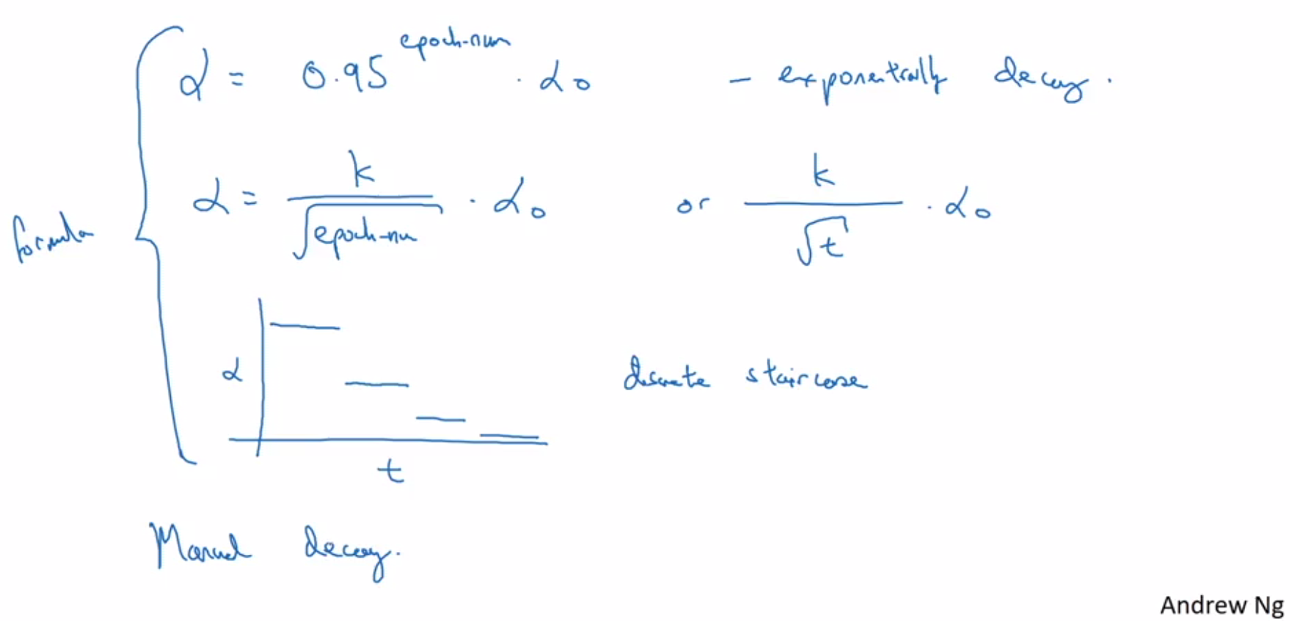
VIF = Variance Inflation Factor

  • In linear regression collinearity can make coefficient unstable
    • There will not be any issue in prediction accuracy but coefficients would be less reliable and p-value would be more
    • Correlation coefficients help us detect correlation between pairs but not the multiple correlation x1 = 2*x3 + 4*x7
    • PCA is one thing, we don’t want to transform variable to keep interpretability intact
    • We want some way to reduce dimensions
  • In VIF, each feature is regression against all other features. If R2 is more which means this feature is correlated with other features.  [0]
    • VIF = 1 / (1 – R2)
    • When R2 reaches 1, VIF reaches infinity
  • We try to remove features for which VIF > 5

vif1

  • Example at [1] shows the use of VIF to reduce no of features.
  • Once we identify high VIF for features we need to reduce it
    • We can do it by eliminating some features
    • How to identify which feature to remove?
      • Check the correlated features for feature having high VIF
      • In the example at [1] weight and BSA were correlated
      • Practically it is easy to measure weight so we kept it
        • So such decision depends on the practical implication
      • There can be the case that one feature is correlated with many others and we might want to remove it      vif2vif2


Reference

[0] : https://www.youtube.com/watch?v=0SBIXgPVex8

[1] : https://newonlinecourses.science.psu.edu/stat501/node/347/


Clustering Metrics

Here are some metric available for validating clustering, explanation of each one is available on sklearn. [0]

If ground truth labels are available:

  • Adjusted Rand Index
  • Mutual Information Based scores
  • Homogeneity, completeness and V-measure
  • Fowlkes-Mallows scores

If not available :

  • Silhouette Coefficient
    • Range (-1,1)
    • 1 means it is similar to data-points in each cluster
  • Calinski-Harabaz Index
  • Davies-Bouldin Index
  • Contingency Matrix


Calculating SSE

It is a sum of distance between each point and its cluster center.

c1

Silhouette Score

It is calculated for each point and then we take an average of it.

c2

c4           c3

a(i) is average distance of a point to other points in same cluster.

b(i) is minimum of above average in for point in other cluster. It given the distance to nearest cluster.

s(i) close to 1 means data point is appropriately clustered. -1 means it is very bad clustered.

Setting s(i) to 0 when cluster size is one ensures that curve is not monotonically decreasing.


Elbow method and Silhouette Analysis

Notebook is available at https://github.com/arcarchit/datastories/blob/master/Silhouette.ipynb

sil1         sil2

Rand Index

  • When cluster labels are available we can use this matrix
  • It basically checks the similarity between two cluster assignments
    • Labels can also be seen as one type of cluster assignment
    • Score basically tells us how similar to cluster assignments are
  • This works by taking pair of points
    • Out of all pairs how many pairs are agreed in both clusters mechanism
    • Agree mean both
      • They are in same cluster in both mechanism
      • They are in different cluster in both mechanism
  • The Rand index has a value between 0 and 1, with 0 indicating that the two data clustering do not agree on any pair of points and 1 indicating that the data clustering are exactly the same

rand_index

  • One drawback of Rand index is that it can given non zero value for random assignment of clusters. To mitigate that there is matrix called Adjusted Rand Index. [2]
    • It specifically does not work when no of clusters are high


Reference

[0] : https://scikit-learn.org/stable/modules/clustering.html

[1] : https://github.com/anthonyng2/udemy-the-complete-machine-learning-course-with-python

[2] : https://davetang.org/muse/2017/09/21/adjusted-rand-index/


Oversampling and Under-sampling

When data is class-imbalanced there is a tendency to predict majority class. One way to tackle this would be apply more weight to minority classes in cost function. Another way is oversampling and under-smapling.

  • Over-sampling makes duplicate copies of minority classes
  • Under sampling randomly removes some samples from majority class
    • This should be used with caution
    • We need to check once that we still remain with enough sample for a given no of features
  • Practically we might want to over sample some classes and under-sample others.


Cross validation

  • Validation set should be taken out from original data[1]
    • We can do the sampling just before training only on training data


Reference

[0] : https://www.kaggle.com/residentmario/undersampling-and-oversampling-imbalanced-data

[1] : https://www.marcoaltini.com/blog/dealing-with-imbalanced-data-undersampling-oversampling-and-proper-cross-validation


Chi Square Test

The chisquare independence test is a procedure for testing if two categorical variables are related in some population.

Here is handwritten example : https://github.com/arcarchit/datastories/blob/master/notes/chi2.pdf

Chi square distribution

  • Chi square distribution
    • Squaring samples from standard normal distribution [0]
    • Distribution changes with degrees of freedom
    • When DoF = 1 it is more concentrated around 0
  • It is distribution is sum of squares
    • When dice is biased sum of squares will be higher. Hence more significant.
    • When it is fair it will be closed to zero. Difference is with expected value.
d1
d2

Chi Square Test for Equality of Proportions

h1

Chi square vs T test

  • When to use which one
  • T-test is used to compare mean of two distributions
  • Chi square is used to check whether observation gathered of categorical data meets the assumption

Chi Square for goodness of fit testing

  • Chi Square Goodness of fit
    • Restaurant example
    • H0 = Percentage given by customer is correct
  • We calculate expected for each cell and calculate chi^2

Chi Square for relationship testing

  • H0 : Variables are independent of each other
  • It helps testing if two categorical variables are related
  • Calculate Chi square statistics by summing all cells and check against degree’s of freedom
  • Examples
    • Hypothesis testing :
      • H0 = Herbs1, Herb2, placebo are same
      • H0 = Herbs do nothing
      • We can’t say herb does nothing
        • We are working on accumulated data here
        • Whereas ANOVA is about variancei1
    • Homogeneity testing  :
      • H0 = Left and Right handed people have same preference for arts, science
      • H0 = Preference of arts/science is independent of natural hand left/right
      • H0 = Variables are independent
      • Filling up table
        • P(STEM | right) = P(STEM)
        • x / 60 = 40/100 => x = 40 * 60 / 100 = 24
        • We can also say that value of cell is product of marginals divide by total
      • Degrees of freedom = (r-1)*(c-1)  = 2 * 1 = 2
i3

References

[0] : https://www.khanacademy.org/math/statistics-probability/inference-categorical-data-chi-square-tests#chi-square-goodness-of-fit-tests

[1] : https://www.khanacademy.org/math/statistics-probability/inference-categorical-data-chi-square-tests#chi-square-goodness-of-fit-tests

[2] : https://biology.stackexchange.com/questions/13486/deciding-between-chi-square-and-t-test

[3] : https://fhssrsc.byu.edu/SitePages/ANOVA,%20t-tests,%20Regression,%20and%20Chi%20Square.aspx

Generative and Discriminative Models

Introduction

In machine learning, there are two broad categories of models: generative models and discriminative models. In this blog post, we will discuss some popular examples of each and their capabilities.

Generative Models

  1. Naive Bayes Classifier
  2. Hidden Markov Models
  3. Latent Dirichlet Allocation
  4. Boltzmann Machine
  5. Gaussian Mixture Model ( Unsupervised clustering)

Generative Models Explanation

Generative models allow us to generate datasets for specific classes, labels, or clusters. They estimate the joint probability distribution P(X, y). An example of this is the Naive Bayes Classifier, where we have a probability associated with each (X, y) pair. For classification, we predict y based on the highest probability given x.

𝑎𝑟𝑔𝑚𝑎𝑥𝑦𝑃(𝑌=𝑦|𝑋=𝑥)=
𝑎𝑟𝑔𝑚𝑎𝑥𝑦𝑃(𝑌=𝑦,𝑋=𝑥)/𝑃(𝑋=𝑥) = 𝑎𝑟𝑔𝑚𝑎𝑥𝑦𝑃(𝑌=𝑦,𝑋=𝑥)/𝑃(𝑋=𝑥)

Generative models offer more than just prediction. They can be used to:

  • Impute missing data
  • Compress datasets
  • Generate unseen data

Discriminative Models

  1. Logistic Regression
  2. Support Vector Machines
  3. Decision Trees

Discriminative Models Explanation

Discriminative models focus on learning the boundaries that separate different classes directly. They do not model the entire joint probability distribution but instead estimate the conditional probability P(y|x). Examples of discriminative models include Logistic Regression, Support Vector Machines, and Decision Trees.

Contrast Analysis

  • At Hypothesis and T-Distribution we discussed about hypothesis testing. We had talked about one sample and two sample t test.
  • Contrast analysis is more general case of that.
  • It allows us to make comparison of combination of groups :
  • Can’t we combine them to form just two groups :
    • We want to preserve individual identity of group
      • Group with large no of samples should not dominate group with small no of samples
  • Examples
    • Groups for which the context at test matches the context during learning (i.e., is the same or is simulated by imaging or photography) will perform better than groups with a different or placebo contexts. [2]
    • Group 1 is different from Group 2-3-4
      • 3 types of smile vs 1 neutral [3]
    • Group 1 and 4 are different from group 2,3


contrast1       contrast2

  • Intuition behind formula of standard error
    • Sum of square of combined group is some of individual SoS when groups are independent
  • α should be equal to desired confidence (0.90, 0.95 etc). It is divided by two because it is two sided


Reference

[1] : http://www.youtube.com/watch?v=yq_yTWK4mNs

[2] : https://pdfs.semanticscholar.org/c0ba/1c28b0e120a459820bfb20d430fa442ebd96.pdf

[3] : http://www.onlinestatbook.com/case_studies_rvls/smiles/index.html

NN : Batch Norm and Softmax Regression

This post is a lecture summary of Week 3 of the deep learning course by Andrew N. G, available at https://www.coursera.org/learn/deep-neural-network/home/welcome.

Hyperparameter Tuning

  • When the number of parameters is large, random search is better than grid search.
  • Grid search is more useful when the number of parameters is small, as it is more systematic.
  • Not all hyperparameters are equally important.
  • Choosing between babysitting one model (“Panda” strategy) or training multiple models in parallel (“Caviar”) depends on the computational resources available.

Batch Normalization

  • Normalizing input features speeds up learning by making the contours more circular.
  • In practice, z[2] is normalized instead of a[2].
  • β and γ are introduced to allow for non-zero mean and non-unit variance.
    • Suppose you have sigmoid activation and you want larger variance to better exploit non-linearity
  • Different β and γ values are used for each layer.
  • In deep learning frameworks, batch normalization is often a single flag.
  • When using normalization, the bias term (b) has no effect and can be eliminated.

screen shot 2019-01-15 at 11.53.57 am

screen shot 2019-01-15 at 12.06.40 pm

  • Batch normalization speeds up training, limits distribution shifts of activation, provides more consistent data to later layers, and has a slight regularization effect.
  • Mean-variance scaling with different β and γ values for each mini-batch introduces noise similar to dropout, challenging later layers to not depend on a single feature.
  • Larger mini-batch sizes result in smaller regularization, but batch normalization is not primarily used for regularization.
  • During scoring, calculate µ and σ using exponentially weighted averages across mini-batches for each layer during training.
  • These averages are running averages and do not require much memory.
  • Use the above values for scoring.

Softmax Regression

  • Softmax regression is a generalization of logistic regression.
  • The output vector has dimensions (C, 1) and uses the “Softmax activation” function.
  • Softmax activation involves taking exponentials and normalizing the values.
softmax_layer
  • When C = 2, softmax reduces to logistic regression.
  • The loss function remains the same: cross-entropy loss.
  • Only one class will have an actual value of 1, following the maximum likelihood function.
loss_function
  • The gradient of the last layer is dz = ŷ – y.
backprop

Optimization for NN

Mini-batch Gradient Descent:

  • Mini-batch gradient descent exhibits oscillations during descent.
  • Choosing mini-batch size:
    • For small training sets (< 2k samples), it is advisable to use batch gradient descent.
    • For larger training sets, mini-batches of sizes such as 64, 128, 256, or 512 are commonly used.
  • Cross-validation helps in finding the right trade-off.
  • Batch gradient descent: More training time is dominated by the processing of a single duration.
  • Stochastic gradient descent: More training time is dominated by the number of iterations required for convergence.
    • Vectorization is lost in the case of stochastic gradient descent.

Exponentially Weighted Moving Averages:

  • Exponentially weighted moving averages are computed using the formulas:
    • Vₜ = 0.9 * Vₜ₋₁ + 0.1 * θₜ
    • Vₜ = β * Vₜ₋₁ + (1 – β) * θₜ
  • Averaging over roughly the last 10 days of temperature is achieved using the factor 1 / (1 – 0.9).
  • Bias correction is necessary to eliminate the bias introduced when initializing with v₀ = 0.
  • The bias correction formula is: Vₜ = (1 – βᵗ) * (β * Vₜ₋₁ + (1 – β) * θₜ)
bias_correction

Gradient Descent with Momentum:

  • Gradient descent with momentum enables slower learning on the vertical axis and faster learning on the horizontal axis.
  • In practice, bias correction is not used after around 10 iterations.
gradient_descent_with_momentum.png

RMSprop:

  • RMSprop is used to handle situations where some dw values can be large.
  • Adding epsilon for numerical stability helps prevent division by zero.
  • Notice is the dw^2 in the formula below
rmsprop

Adam Optimization:

  • Adam optimization, short for Adaptive Moment Estimation, is one of the algorithms that works well across domains.
  • Default values commonly used for β₁ (0.9), β₂ (0.999), and ε (10^-8)
adam

Learning Rate Decay:

  • 1 epoch refers to one pass through the entire data.
  • In the case of mini-batches, one epoch can involve multiple iterations.
  • Different formulas are used for learning rate decay
learning_rate_decay.png

Local Optima:

  • Most points with zero gradient are not local optima but rather saddle points, especially in high-dimensional spaces.
  • Local optima are generally not observed due to the high dimensionality.
  • Plateaus can be problematic, with very small gradients leading to slower learning.

Inverted Dropout

This post is a lecture summary of the deep learning course by Andrew N. G, available at https://www.coursera.org/learn/deep-neural-network/home/welcome.

During Training:

  • Neurons are dropped out by setting them to zero.
  • The activation is adjusted by dividing it with the keep probability.
  • The expected value of z[4] (as shown in the screenshot below) should not be altered.
inverted_dropout

During Scoring:

  • If “inverted dropout” is used, no additional steps are necessary.
  • Other dropout techniques may require some computations.

Intuition:

  • Dropping out neurons causes inputs to the unit to be randomly dropped.
  • This prevents the unit from relying too heavily on a single feature and encourages it to distribute weights across multiple features.
  • Different layers can have different keep probabilities.

Side Effect:

  • The cost function is not well defined.
  • It’s not possible to check if the cost is consistently decreasing every iteration.
  • A debugging tool is used to address this issue.

Solution:

  • First, verify that everything is functioning correctly without dropout.
  • Then, gradually introduce dropout.

———————————————————————–

Other Regularization Techniques

  • Data augmentation, such as horizontal flipping, random cropping, and transformations.
  • Early stopping: Stop training at a certain iteration (e.g., 7k instead of 10k) based on the error observed on the development set.

Downside

  • Balancing optimization and avoiding overfitting can be challenging.
  • Mixing both objectives requires careful consideration.

Advantage

  • Unlike L2 regularization, dropout does not necessitate trying different lambda values repeatedly.

Hidden Markov Models

From a Clustering Perspective

This section summarizes a lecture from the University of Washington [0] on clustering time series data, considering the significance of both the data and indices.

Other potential applications include:

  1. Honey bee dance: Bees switch from one dance to another to convey messages.
  2. Conference conversations: Segmenting speaker assignments based on the spoken turns.
  3. Gym exercises: Identifying exercises from pulse rate data as people switch between activities.

Model

The following screenshots are from a YouTube video [1] by the Mathematical Monk, illustrating the model:

Suppose you’re developing handwriting recognition and need to recognize a hidden variable.

The prediction for “i” depends solely on the previous character being “h,” disregarding how “h” was written.

hmm_concept
hmm_parameters

Code and Notebook

You can find the code and notebook at the following GitHub link [2], which extensively explains:

  1. The structure of the model.
  2. The forward algorithm for calculating the likelihood of a given observation.
  3. The backward algorithm for finding the most probable state sequence given an observation (also known as decoding).
  4. The forward-backward algorithm for inferring model parameters from a set of observed sequences.

References

[0] : https://www.coursera.org/learn/ml-clustering-and-retrieval/home/welcome

[1] : https://www.youtube.com/watch?v=TPRoLreU9lA

[2] : https://github.com/arcarchit/datastories/blob/master/hmm.ipynb

[3] : https://web.stanford.edu/~jurafsky/slp3/A.pdf