On LDA, QDA

{In practice it is used more for classification than for regression}

This resemble gaussian mixture models in that you git one gaussian for each class. 
Don't forget one important difference though. LDA is supervised, Mixture models are unsupervised.

Linear Discriminant Analysis (LDA)

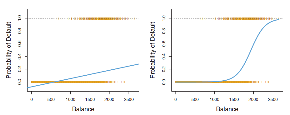
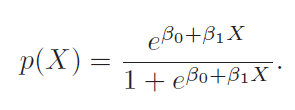
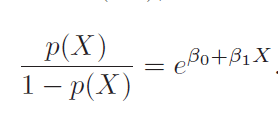
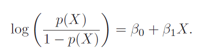
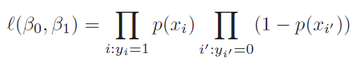
In logistic regression (LR), we estimate the posterior probability directly. In LDA we estimate likelihood and then use Bayes theorem. Calculating posterior using bayes theorem is easy in case of classification because hypothesis space is limited.

1234

Equation 2 computes probability of class k given x. This is a posterior instead of just point estimates.

Equation 4 is derived from equation 3 only. Probability(k) would be highest for the class for which Delta(k) will be highest.

LDA estimates mean and variance from data and uses equation 4 for classification.

5

We also need to estimate π_k, which I think would be n_k/N.


Assumptions made:

  • f(x) is normal
  • Variance(sigma) is same for all classes


When more than one predictor, we go for multivariate gaussian

67

Some comparisons

  • Compare this with mixture models, where there is a responsibility vector for each sample
    • There labels are not available (unsupervised learning) and hence is solved by EM (Expectation Maximization)
  • Compare this with naive bayes, there assumption is each feature is independent
    • Here we have parameter for each (class, feature), there we have parameter for each feature
    • Also here f captures probability of class (k) given x, there after bayes rules we calculate probability of x given class k
    • Hence the name naive bayes
    • Here we have joint distribution (multivariate gaussian, there it is independent distribution for each features)
    • Both LDA and navie bayes try to calculate posterior while logistic regression maximizes likelihood function


Quadratic Descriminant Analysis (QDA)

Unlike LDA, QDA assumes that each class has its own covariance matrix. It is called quadratic because below function is quadratic of x.

8

When to use LDA, QDA

  • This is related to bias variance trade-off
  • For p predict and k classes
    • LDA estimates k*p parameters
    • QDA estimates additional k*p*(p+1)/2 parameters
  • So LDA has much lower variance and classifier built can suffer from high bias
  • LDA should be used when number of training sample are less, because we want to avoid high variance problem
  • QDA has high variance, so it should be used when number of training samples are more
    • Another scenario would the case when common covariance matrix among K classes is untenable


A note on Fisher’s Linear Discriminant Analysis

  • It is simply LDA in case of two classes.
  • We can derive this similarity mathematically.
  • In literature we found it from the perspective that it project data on a line which achieves maximum separation
  • We can state without loss of generality that LDA also provides low dimensional view on data


Math

  • We want to project 2-D data on a line which
    • maximizes the difference between projected mean
    • minimizes within class variance
  • Such a direction (w) can be found by maximizing fisher criterion (J)

fisher1fisher2fisher3

fisher4fisher5fisher6fisher7


Classification – One vs Rest and One vs One

In the blog post on Cost Function And Hypothesis for LR we noted that LR (Logistic Regression) inherently models binary classification. Here we will describe two approaches used to extend it for multiclass classification.

One vs Rest approach takes one class as positive and rest all as negative and trains the classifier. So for the data having n-classes it trains n classifiers. Now in the scoring phase all the n-classifier predicts probability of particular class and class with highest probability is selected.

One vs One considers each binary pair of classes and trains classifier on subset of data containing those classes. So it trains total n*(n-1)/2 classes. During the classification phases each classifier predicts one class. (This is contrast to one vs rest where each classifier predicts probability). And the class which has been predicted most is the answer.

Example

For example consider four class problem having classes A, B, C, and D.

One vs Rest

  • Models classifiers_A, classifier_B, classifier_C and classifier_D
  • During prediction here is the probability we get:
    • classifier_A = 40% = prob(class A)
    • classifier_B = 30%
    • classifier_C = 60%
    • classifier_D = 50%
  • We assign it class B
  • Note that Summation might not be come out to 1
    • Prob(class A) + Prob(class B) + Prob(class C)

One vs One

  • We train total six classifier with subset of data containing classes involved
    • classifier_AB
    • classifier_AC
    • classifier_AD
    • classifier_BC
    • classifier_BD
    • classifier_CD
  • And during classification
    • classifier_AB assigns class A
    • classifier_AC assigns class A
    • classifier_AD assigns class A
    • classifier_BC assigns class B
    • classifier_BD assigns class D
    • classifier_CD assigns class C
  • We assign it to class A
  • How do we estimate Prob(class A) ?
    • Somewhat complicated

More notes

  • One vs rest trains less no of classifier and hence is faster overall and hence is usually prefered
  • Single classifier in one vs one uses subset of data, so single classifier is faster for one vs one
  • One vs one is less prone to imbalance in dataset (dominance of particular classes)

Inconsistency

  • What if two class gets equal vote in the case of one vs one case
  • What if probability are almost close to equal in case of one vs rest
  • We will discuss this issue in further blog posts

On Classification Accuracy

Edit : Extended post is available here

Some Scenarios

  • In finance default is failure to meet the legal obligation of loan. Given some data we want to classify whether the person will be defaulter or not.
    • Suppose our training data-set is imbalanced. Out of 10k samples only 300 are defaulters. (3%)
    • Classifier in the following table is good at classifying non defaulters but not good at classifying defaulters (which is more important for credit card company)
    • Assume what if out of 300 defaulters 250 are classified as non defaulters and given the credit card
  • Doctors want to conduct a test whether a patient has cancer or not.
    • Popular terms in medical field are sensitivity and specificity
    • Instead of trying to classify person as defaulter, here we classify if patient has cancer.
    • Sensitivity = 81/333 = 24 %
    • Specificity = 9644/9667 = 99 %
    • Every medical test thrives to achieve 100% in both sensitivity and specificity.
  • In information retriever we want to know how many % of relevant pages we were able to retrieve.
    • TP = 81
    • FP = 23
    • TN = 9644
    • FN = 252
    • Precision = 81/104= 77%
    • Recall = 81/333= sensitivity = 24%

Example

1

  • Formulas:
    • Precision = TP/(TP+FP)
    • Recall = TP/(TP+FN)
    • Sensitivity = TP/(TP+FN)
    • Specificity = TN/(TN+FP)
    • Recall and sensitivity are same

Solution is to change the threshold

  • Earlier we were assigning person to default if probability is more than 50%
  • Now we want to assign more person as defaulter
  • So we will assign them to defaulter when probability is more than 20%
  • This will incorrectly classify non-defaulters to defaulters but that is less concerned compared to assigning defaulter to non-defaulter
    • This will also increase the overall error rate, which is still okay

ROC and AUC

  • We can always increase sensitivity by classifying all samples as positive
  • We can increase specificity by classifying all samples as negative
  • ROC plot (sensitivity) vs (1-specificity)
    • That is TP vs FP
    • And also precision vs recall
  • ROC = Receiver operating characteristic
  • It is good to have ROC curve on top left
    • Better classifier
    • Accurate test
  • And ROC curve close to 45 degree represents less accurate test
  • AUC = Area Under Curve
    • Area under ROC curve
  • Ideal value for AUC is 1
  • AUC of 0.5 (45 degree line) represents a random classifier


How to plot ROC?
  • Change the probability threshold from 0 to 1 and measure sensitivity and specificity. If specificity keeps on decreasing ((100-specificity) keeps on increasing) as sensitivity increase it is a bad classifier.
  • For random classifier ROC is 45 degree line
    • You draw random number between (0, 1)
    • Classify it based on threshold
    • So threshold is there
    • But while building classifier we want to do better than drawing random probability between (0, 1). We also want to consider features into account while drawing between (0, 1)
  • Can AUC be less than 0.5? I don’t think so.
    • Complementing the output will bring it to other side of line anyway.
  • What if I classified all of them as positive?
    • That means you are taking all 1. You can not plot ROC with that.

auc

Threshold selection

  • Unless there is special business requirement (as in credit card defaulters) we want to select a threshold which maximizes TP while minimizing FP
  • There are two methods to do that:
    • Point which is closest to (0, 1) in ROC curve
    • Youden Index
      • Point which maximizes vertical distance from line of equality (45 degree line)
      • We can derive that this is the point which maximizes (sensitivity + specificity)


AUC vs overall accuracy as comparison metric

  • AUC helps us understand how much our classifier is away from random guess, which accuracy can not tell
  • Accuracy is measured at particular threshold while AUC requires moving threshold from 0 to 1


F score

  • We know that recall and sensitivity are same, but precision and specificity are not same
  • While medical field is more concerned about specificity, information retrieval is more concerned about precision
  • So they came up with F score which is harmonic mean of precision and recall
  • AUC helps us maximizing sensitivity and specificity simultaneously while F score helps us maximizing precision and recall simultaneously
  • Beta in f score helps providing weight to precision and recall.
  • Harmonic mean can not be made arbitrarily large while changing some values to bigger one and leaving at least one unchanged. It is maximizes when all elements are increased.
    • x = 0, y = 1 will give 0.5 in arithmetic mean but is zero for harmonic mean

h_mean

harmonic mean


f_score.PNG

References

Assessing and Comparing Classifier Performance with ROC Curves

Click to access roccurve.pdf

https://www.medcalc.org/manual/roc-curves.php

https://en.wikipedia.org/wiki/F1_score

An Introduction to Statistical Learning – http://www-bcf.usc.edu/~gareth/ISL/

https://stats.stackexchange.com/questions/221997/why-f-beta-score-define-beta-like-that

https://en.wikipedia.org/wiki/Harmonic_mean

Cost Function And Hypothesis for Logistic Regression

Hypothesis

We want a hypothesis that is bounded between zero and one, regression hypothesis line extends beyond this limits. Hypothesis here also represents probability of observing an outcome.

1

Hypothesis by ISLR and Andrew N.G :

Odds and log-odds/logit

Log of odd is also called logit. So above is logit(p(x)) = b0 + b1X.

In terms of GLM we call it a logic link function. Logit has a property of broadcasting [0,1] range to [-inf, inf]. Log does not have that property.

In regression beta1 given average change in y for unit change in x. But here it says unit increase in x changes log-odds by beta1. It multiplies odds by exp(beta1) and hence depends on current value of odds and therefor is not linear.


Cost Function

For ISLR perspective it is likelihood that we want to maximize.

9

Andre N.G looks it from the perspective of modifying cost function of linear regression.

8

As we can see that Andrew N.G cost function is same as maximizing log likelihood of ISLR.

Least square in case of linear regression is special case of maximum likelihood. We know that derivation where we assume likelihood to be gaussian.

Logistic Regression For well separated classes

MLE estimation becomes unstable when classes are well separated. While this is acceptable for classification tasks, it is not ideal for risk estimation. Regularization techniques can help avoid this instability. Support Vector Machines (SVM) also perform well for well-separated classes. As shown in figure below[1], the intercept of the sigmoid function reaches -inf, and the slope reaches inf. This allows the slope to come from an infinitely weighted feature.

enter image description here

Why Can’t we use square loss ?

  • Labels (+1, and -1)
  • Prediction : +1 when w*x > 0 else -1
  • Consider scenario [2]
    • label +1
    • w*x = 100
    • Prediction is correct
    • Still we add it to loss (100-1)^2
  • Solutions are hinge loss and logistic loss
  • Why is not logistic loss not 0 for correct prediction ?
    • There are more training samples. We want to find parameter (w) such that it balances all of them
    • If we make it 0 positive examples would no longer contribute to loss (like SVM)
      • That’s why hinge loss create support vectors. More about that on SVM’s blog post
    • Also this is the property which will make coefficient (w) higher for well separated classes
      • To control that we use regularisation
      • Regularisation is while training, not while prediction, we are just changing loss function
      • Predict is still +1 is w*x > 0 else -1

Why can’t we use step loss ?

  • When we are incurring loss, we also want to know which direction to go to reduce loss.
  • Gradient/slope is what provide this information. [2]
  • Step loss (0-1) has zero gradient

Reference

[1] https://stats.stackexchange.com/questions/254124/why-does-logistic-regression-become-unstable-when-classes-are-well-separated

[2] Notes of different loss function is taken from Mike Galbart’s course – https://github.com/UBC-CS/cpsc340/blob/master/lectures/L19demo.ipynb