Interpretation of Multiple Regression Coefficients

  • In case of simple linear regression with one variable we interpret slop coefficient as follows
    • y = b0*x0 + c
    • b0 is increase in y for unit increase in x0
  • In case of multiple regression:
    • y = b0*x0 + b1*x1 + c
    • b0 is increase in y for unit increase in x0 keeping x1 constant


Implication of keeping other variable constant:

  • Consider
    • house_price = b0 * no_of_bedrooms + c       ….. (1)
    • house_price = b0 * no_of_bedrooms + b1*square_feet + c     …..(2)
  • In (1) there are high chances that b0 will be positive
  • In (2) it can be negative
    • If you increase no of bedrooms keeping square feet constant each room will be smaller
    • This may decrease house price


Reference :

Coursera course on regression by University of Washington DC : https://www.coursera.org/specializations/machine-learning


Grubb’s Test for Anomaly Detection

Problem Statement:

We are receiving time series of count data everyday and we want to detect whenever there is drastic change in this count.


Grubb’s test assumes a t-distribution of input and find out the outliers for required confidence interval. We remove this outlier and repeat the test again. Here is the pseudo code:


Grubbs Test(X, p-val=0.05):
    Repeat :
        Z <- zscore(X)
        n < len(X)
        zi, index <- max(abs(Z)), index(max(abs(Z)))
        if zi > threshold(N, p-val):
            remove X[index] 
        else:
            break


Traditionally Grubb’s tests has a alternate hypothesis that exactly one outlier is present in data. In above we modified it get all possible outliers.


Test Hypothesis
Grubb’s Test H0: There are no outliers in the data set
Ha: There is exactly one outlier in the data
Tietjen-Moore test H0: There are no outliers in the data set
Ha: There are exactly k outliers
Generalized ESD test H0: There are no outliers in the data set
Ha: There are up to r outliers


Above can be extended to two sided tests as well.


We had followed this in time series based anomaly detection and following approach were considered for pre processing before applying Grubb’s test:

  • Raw Count (No processing)
  • Residuals after STL decomposition
  • Residuals after fitting ARIMA

In our case raw count had worked well enough.


Reference:

https://www.itl.nist.gov/div898/handbook/eda/section3/eda35h1.htm

Github Gist


Ensemble, Bagging and Boosting

Ensembling is a method of combining more than one models to generate a final output.(Reference [1])

There are two ways of doing that:

  1. Bagging
  2. Boosting


Bagging Boosting
  • We take subset of data and train different models
  • Example Random forest
    • It takes subset of data as well as subset of features
  • Pros of random forest
    • Handles high dimensions
    • Handles missing values
  • Cons of random forest
    • It won’t give precise value regression because final value is mean from subset tress
    • None the less people are using it for regression depending upon domain
  • We train different model on with same data. Each sample is assigned different weight in each iteration
  • Example AdaBoost, XgBoost
  • Pros of XgBoost
    • Supports different loss function
    • Works well with interactions
  • Cons of XbBoost
    • Prone to overfitting
    • Tuning of hyper parameters is critical


Pros-cons of bagging vs boosting:

  • Bagging is easy to parallelize and hence training is faster
  • Boosting is more efficient for fixed no of iterations (classifiers)


AdaBoost vs XgBoost

Reference : [2]

ada_vs_xg

Quote from Tianqi Chen, one of the developers of XGBoost:

Adaboost and gradboosting [XGBoost] are two different ways to derive boosters. Both are generic. I like gradboosting better because it works for generic loss functions, while adaboost is derived mainly for classification with exponential loss.


Reference :

[1] https://towardsdatascience.com/decision-tree-ensembles-bagging-and-boosting-266a8ba60fd9

[2] https://www.packtpub.com/mapt/book/big_data_and_business_intelligence/9781788295758/4/ch04lvl1sec34/comparison-between-adaboosting-versus-gradient-boosting


AdaBoost

  • AdaBoost stands for adaptive boosting
  • Boosting is a technique for creating better classifier form several regular/weak/base classifiers
  • Thought:
    • We want to train second classifier in such a way that training data has more samples for the case where first classifier was wrong
    • Third classifier will have more samples where first and second classifier contradicts
  • How do we accomplish above:
    • We assign weights to each sample
      • This weights will be used in error function for each sample
      • Error function would be sum of weights of incorrectly classified samples
      • This weights keep changing in each iteration
    • We also assign wight to each base (weak) classifier (α In below algorithm)
      • Formula for calculating α below is valid for binary classification
        • It will be different for multi class classification
  • When do we stop iteration ?
    • Combined classifier is predicting all sample correctly
    • No more base classifier left
  • Most machine learning algorithms allows to apply weight to data
    • In logistic regression we can multiply weight in error fucntion
    • In decision tree, classification error can be calculated by summing weights of missclassified samples


adboost


Formulations in above algorithm:

  • Formula of α
    • if ε=0.5 then α=0. It is just a random chance classifier.
    • Else it can positive/negative.
    • ε < 0.5 => negative α => we invert the prediction in weighted average
  • Formula of D_(t+1)(i)
    • y*h is just a sign
      • y and h are  {-1, 1}
      • y*h will be positive for correct prediction
    • Why it is function of ε
      • Random classifier updating weights does not make sense
  • By Z_t we are normalizing weights, which ensures numerical stability


Adaboost Theorem

  • Error -> 0 as no of iteration -> infinity at certain condition
  • Condition is here is that each learner has error < 0.5
  • Each iteration means adding one weak learner


Over-fitting

  • Contrary to weak classifier (decision stumps) we saw that rate of increase test error is less with boosting
  • However no of iteration still should be selected via cross validation for small data-set and validation for large data-set


References:

Click to access MIT6_034F10_boosting.pdf

Click to access msri.pdf


IID Assumption

This is an interesting thread on the topic : https://stats.stackexchange.com/questions/213464/on-the-importance-of-the-i-i-d-assumption-in-statistical-learning


Some notes:


1) Method of cross validation changes based in i.i.d assumption.

2)

tom

Looking at the last three equation, p(D/h) = p((d1, d2, d3)/h) can be reduced to multiplication only when d1, d2, d3 are independent.


Panel Data And Analysis

From Wikipedia

In statistics and econometrics, panel data or longitudinal data[1][2] are multi-dimensional data involving measurements over time. Panel data contain observations of multiple phenomena obtained over multiple time periods for the same firms or individuals

Time series and cross-sectional data can be thought of as special cases of panel data that are in one dimension only (one panel member or individual for the former, one time point for the latter).

A study that uses panel data is called a longitudinal study or panel study.


Cross sectional data:

Cross-sectional data, or a cross section of a study population, in statistics and econometrics is a type of data collected by observing many subjects (such as individuals, firms, countries, or regions) at the same point of time, or without regard to differences in time.

Analysis of cross-sectional data usually consists of comparing the differences among the subjects.


Examples


Panel Data

panel

Cross Sectional Data

cs

Time Series

ts

Regression Trees

Figure below shows how decision tree creates rectangle in predictor space:

As we have describe classification tree, the only difference here is how to come up with output instead of label and how to define a metric other than entropy/gini.

For output it uses the mean of leaves.

For metric CART methodology uses simple SSE.

  • SSE = ∑ (y_i – y1)² + ∑(y_i – y2)²
    • where y1 and y2 are means of two newly crated groups.
    • It is simple sum of squares, not standard deviation 
    • While deriving R2 in linear recession we were concerned with sum of squares
    • Ward linkage criterion in hierarchical clustering also uses difference in sum of squares
  • diff = SSE_before – SSE_after
    • We choose a predictor which minimizes SSE the most.
    • diff is highest

My hand-coded regression tree is available at : https://github.com/arcarchit/datastories/tree/master/regression_tree

Reference

Applied predictive modeling by Max Kuhn and Kjell Johnson

Classification Trees

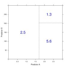
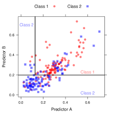
How classification Tree creates Rectangle in Predictor Space

Criterion for Choosing the Splitting Predictor

When deciding which predictor to split on, we need to consider different types of predictors: continuous, binary, and categorical. In this post, we will focus on continuous and binary predictors.

For categorical predictors, one approach is to use the “one vs rest” strategy. We evaluate each category separately and observe which one reduces the randomness the most when split.

In the case of a continuous predictor, we first sort the values and then select the midpoint as the split point.

To keep our decision tree simple, it’s ideal to have a small tree size. Therefore, at each step, we should choose the split that leads to the purest child nodes.

Two commonly used criteria for measuring impurity are Gini and Entropy. It’s important to note that these criteria are not directly used to select the predictor to split on. Instead, we calculate the difference in impurity before and after splitting.

When computing Gini or entropy after splitting, we apply weights to both splits to account for their proportions.

Multi-class

Decision tree can naturally handle multi class problem as entropy and gini can be calculated for multi-class.

Entropy

  • Formula:
    • H = ∑ -p * log(p)
  • About :
    • Randomness
    • Information Carries
    • Highest when p=0.5
    • Higher Entropy => Higher Randomness => Carries more information
    • After splitting we want entropy to reduce
  • Initial :
    • n0 positive and m0 negative sample
    • g0 = (n+m) total samples
  • After Splitting
    • Group 1:
      • n1 positive
      • m1 negative
      • g1 = (n1 + m1) total
    • Group 2:
      • n2 positive
      • m2 negative
      • g2 = (n2 + m2) total
  • Before Entropy :
    • H_before =  -(n0/g0) log(n0/g0) – (m0/g0)log(m0/g0)
  • After Entropy :
    • H1 = -(n1/g1) log(n1/g1) – (m1/g1)log(m1/g1)
    • H2 = -(n2/g2) log(n2/g2) – (m2/g2)log(m2/g2)
    • H_after = (g1/g0) * H1 + (g2/g0)*H2
  • diff = H_before – H_after
  • Select a predictor for which diff is highest and split on it
    • Which means we are selecting a predictor which reduces randomness more
    • Which also mean we are selecting a predictor which reduces information more
      • So we are selecting a variable which carries more information
        • More important feature

Gini

  • Gini for 2 class :
    • G = p1 * (1-p1) + p2 * (1 – p2)
    • Using (p1 + p2 = 1) we can derive that G = 2*p1*p2
  • Gini in general:
    • G = ∑ p * (1 – p) = 1 – ∑ p²
  • Like entropy gini is maximum when p1 = p2 = 0.5
    • In this case nodes are least pure
  • Gini is a measure of impurity which we want to reduce by splitting on predictor
  • diff = G_before – G_after
    • We will select a predictor for which diff is highest

Entropy vs Gini

  • Given a choice gini will be better as computing log is costlier.
  • Both of them are better than “classification error as metric” [1]
    • Which would be selecting majority class for calculating classification error
    • It is useful while pruning but not while growing the tree

ROC Curve

  • ROC curve can be constructed easily for classifier which outputs ranking.
  • On the contrary decision tree outputs label
  • However to get a ROC we can use workaround. Each leaf node will have some positive and negative samples and we can calculate probability as (# positive / # total).
  • Then we can change the threshold and plot ROC.

Regularization

Regularization in decision tree will be explained in separate blog in detail, but here is the list of candidate techniques.

  1. limit max. depth of trees
  2. Cost complexity pruning
  3. ensembles / bag more than just 1 tree
  4. set stricter stopping criterion on when to split a node further (e.g. min gain, number of samples etc.)

Reference

[0] : Applied predictive modeling by Max Kuhn and Kjell Johnson

[1] : https://github.com/rasbt/python-machine-learning-book/blob/master/faq/decision-tree-binary.md

Q-Learning

Value Function

This represents value of a given state for the policy π.

q1

Optimal Policy

q2

Learning Via Value Function is not possible when we don’t know immediate rewards and next state. If they are known we can use dynamic programming methods described at Dynamic Programming for RL.

q3

Q function

q41

q42

How it solve the problem of unknown reward and next state functions?

  • To calculate value function we need to know immediate reward for next state and probability of moving into next state
  • In Q learning we are don’t need them
    • We just take best action, then observe the reward for whichever state we go in.
    • It is possible to know reward after taking action, not before that.


Training Rule for Q

We initialize Q table with random values and keep updating it on each action based on reward get.

q5

We have trained grid world with above equation. Notebook is available at [2]. One thing to note in that code is that, we don’t need backup. We don’t need to update entire q table simultaneously. We can calculate new value for once cell and write it at once.

Also [1] is a very good resource. It shows changes in the Q-update equation in non deterministic world. (Reward and next state are non deterministic).

qq3

And also derives TD updates (Temporal Difference)

qq4


Convergence Conditions

  • System is deterministic MDP (Markov Decision Process)
  • Immediate reward values are bounded
  • Agent visit every state action pair infinitely often


Derivation for Convergence

q6

Experimental Strategies

  • We also need to do exploration
  • So we pick up action with a probability such that
    • action having more Q value has higher probability
  • One way to formulate this is as follows where in value of k control exploration-exploitation trade-off.
    • Initially k is small (exploration) and then is slowly increased (exploitation)

q7


How can we speed up Updating Sequence

  • Strategy 1
    • Consider the case for single absorbing goal state case. (What it means that if agent’s goal is to reach particular state) and initially all (q,a) pairs are initialized with 0.
    • So only one (q,a) pair will be update when we reach to reward state,
    • To speed up things, we can store intermediate state and action and then update backward till origin once we reach reward state.
    • Of course this will increase memory requirement
  • Strategy 2
    • Store immediate reward of past along with state-action pair and retrain periodically
    • If one Q(s, a) changes it will help change others as well
  • Strategy 3
    • If performing real environment action in environment is difficult we can perform simulation


Reference :

[0] Machine Learning by Tom Mitchell

[1] http://www.cs.cmu.edu/afs/cs.cmu.edu/project/theo-20/www/mlbook/ch13.pdf

[2] https://github.com/arcarchit/datastories/blob/master/RL_GridWorld.ipynb