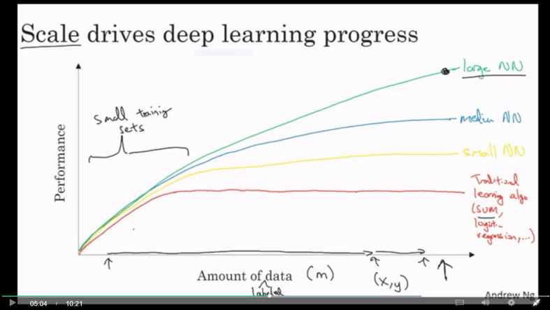
I recently started Andrew Ng’s specialization on deep learning and found these two interesting points :
One is about how performance of algorithm changes with the amount of data. Traditional algorithms have limits but Deep neural network has more advantages.
Also for the small amount of data traditional algorithms may win over neural nets with good feature engineering.
Second reason is that deep learning requires data, computation and efficient algorithms. Recent years have seen significant advancement in algorithm to increase computation efficiency. For example sigmoid to ReLU was an algorithmic change which allowed gradient to converge faster.
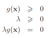
Suppose p is the solution of primal problem and d the dual problem.
If original problem is minimization, we are interested in lower bound (d) such that d<p. We want to find maximum value of d and dual problem becomes maximization problem.
If original problem is maximization, we are interested in finding upper bound (d) such that p<d. We want to find minimum value of d and dual problem become minimization problem.
Dual problem is always convex irrespective of primal problem.
d<p is weak duality, while d=p is strong duality.
If primal problem is convex strong duality generally holds.
We rarely heard of nonparametric tests while reading standard statistical books. However there are some scenarios where they should be used instead of parametric tests. [1] has beautiful blog about it, I am putting just a summary from that.
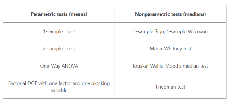
Different Tests
Table below displays various tests, I have verified that all of these tests are available in python stats package.
When to Use Parametric Tests
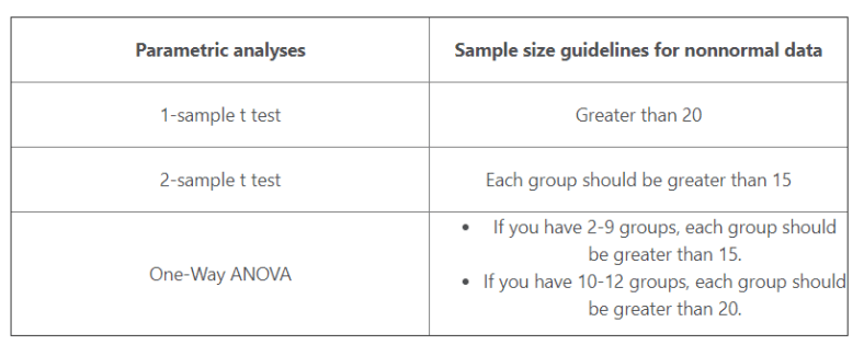
Parametric tests can perform well with skewed and nonnormal distributions
It is important to follow guidance in the sample size of data as shown in table below
Parametric tests can perform well when the spread/variance of each group is different
It has Statistical power
Reasons to Use Nonparametric Tests
Your area of study is better represented by the median
Income distribution is skewed and median is more useful than mean
Few billionaires can boost up the mean significantly
You have a very small sample size
Even less than what is mentioned in table above
You have ordinal data, ranked data, or outliers that you can’t remove
Σ being a positive definite ensure quadratic bowl is downwards
σ2 also being positive ensure that parabola is downwards
On Covariance Matrix
Definition of covariance between two vectors:
When we have more than two variable we present them in matrix form. So covariance matrix will look like
Above is very similar to how we compute sigma^2 in 1-D = (x – mu)^2
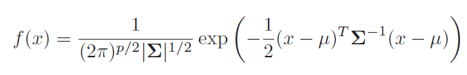
Formula of multivariate gaussian distribution demands Σ to be singular and symmetric positive semidefinite, which in terms means sigma will be symmetric positive semidefinite.
For some data above demands might not meet
Side Note
Covariance is directional measure
Correlation is scaled measure
We normalise by individual variance
Derivations
Following derivations are available at [0]:
We can prove[0] that when covariance matrix is diagonal (i.e there is variables are independent) multivariate gaussian distribution is simply multiplication of single gaussian distribution of each variable.
It was derived that shape of isocontours (figure 1) is elliptical and axis length is proportional to individual variance of that variable
Above is true even when covariance matrix is not diagonal and for dimension n>2 (ellipsoids)
First part above says that bi-variant destitution can be generated from two standard normal distribution z = N(0,1).
For any given k-variant Gaussian we can represent it as linear combination of k standard normal distribution. One simpler way to find these coefficient is Cholesky decomposition. Theorem 1 below stats the same thing.
This has a reference from [1].
Linear Transformation Interpretation
This was proved in two steps [0]:
Step-1 : Factorizing covariance matrix
Step-2 : Change of variables, which we apply to density function
On Practical Example
Height, wight and waist size of men in US (Of course it weight can be negative, so it is approximately normal)
Understanding probability rules and solving tricky probability questions can be challenging. In this blog post, we will explore key probability rules and discuss solutions to some intriguing questions.
Probability Rules:
Joint Distribution: The probability of events X and Y occurring together is denoted as p(X, Y) and is known as the joint distribution.
Conditional Distribution: The probability of event X given event Y is denoted as p(X/Y) and is known as the conditional distribution.
Marginal Distribution: The probability of event X, with event Y marginalized out, is denoted as p(X) and is known as the marginal distribution.
Operations:
Making Conditional Distribution: To obtain the conditional distribution, normalization is required.
Marginalization: Marginalization does not require normalization.
Note: It is not possible to derive the conditional distribution from the joint distribution solely through integration. There is no direct relationship between them.
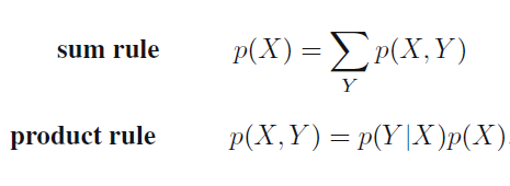
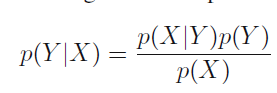
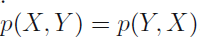
There are just two rules for probability. Sum rule and product rules. And then there is Bayes theorem. Bayes theorem can be derived from product rule and the fact that P(x,y) = P(y,x)
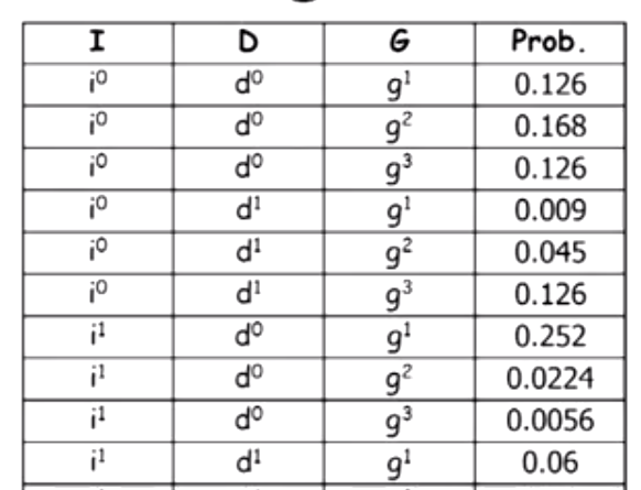
We might want to look at a table like below and calculate joint and conditional distribution and marginalized out one of the variable. [1]
Probability Tricky Question
This questions are taken from [2]. One key to solve this question is write down the sample space and keep eliminating choices. Don’t conclude in hurry.
Q1 : A man comes up to you on the street and says: I have two children. At least one of them is a boy. What is the probability that the other child is also a boy?
Q2 : I have two kids, what are the odds I have 2 boys?
Q3 : A man comes up to you on the street and says: I have two children. The older one is a boy. What is the probability that the other child is also a boy?
Q4 : A man comes up to you on the street and says: I have two children. One is the boy standing here next to me. What is the probability that the other child is also a boy?
Q5 : Q. A man comes up to you on the street and says: I have two children. One of them is a boy who was born in the summer. What is the probability that the other child is also a boy? (There are four seasons : spring, summer, fall, winter)[0]
Ans1 : (1/3)
P(BG) is 1/2 and p(BB) = 1/4 in the universe
Ans2 : (1/4)
Ans3 : (1/2)
Ans4 : (1/2)
Ans5 : (7/15) [0]
Compare Q1 and Q5. Odd increases. Being born in summer is rare thing. If that rare thing has occurred there are higher chances of having two boys.
A bag contains (x) one rupee coins and (y) 50 paise coins. Four coins are taken from the bag and put away. If a coin is now taken at random from the bag, what is the probability that it is a one rupee coin?
Ans is x/(x+y). It will remain same if we take either 1/2/3/4/5 coins because we don’t know which coin has been withdrawn. It is like trying out all possibilities and when we sum, it would come out as 1 only. [4]
The probability of a car passing a certain intersection in a 20 minute windows is 0.9. What is the probability of a car passing the intersection in a 5 minute window? (Assuming a constant probability throughout)
Ans : 0.4377 [5]
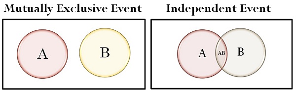
Independent Events
Mutually exclusive events means dependent event
For independent event = P(A/B) = P(A)
For mutually exclusive event if we know B has occurred, A will never occur.
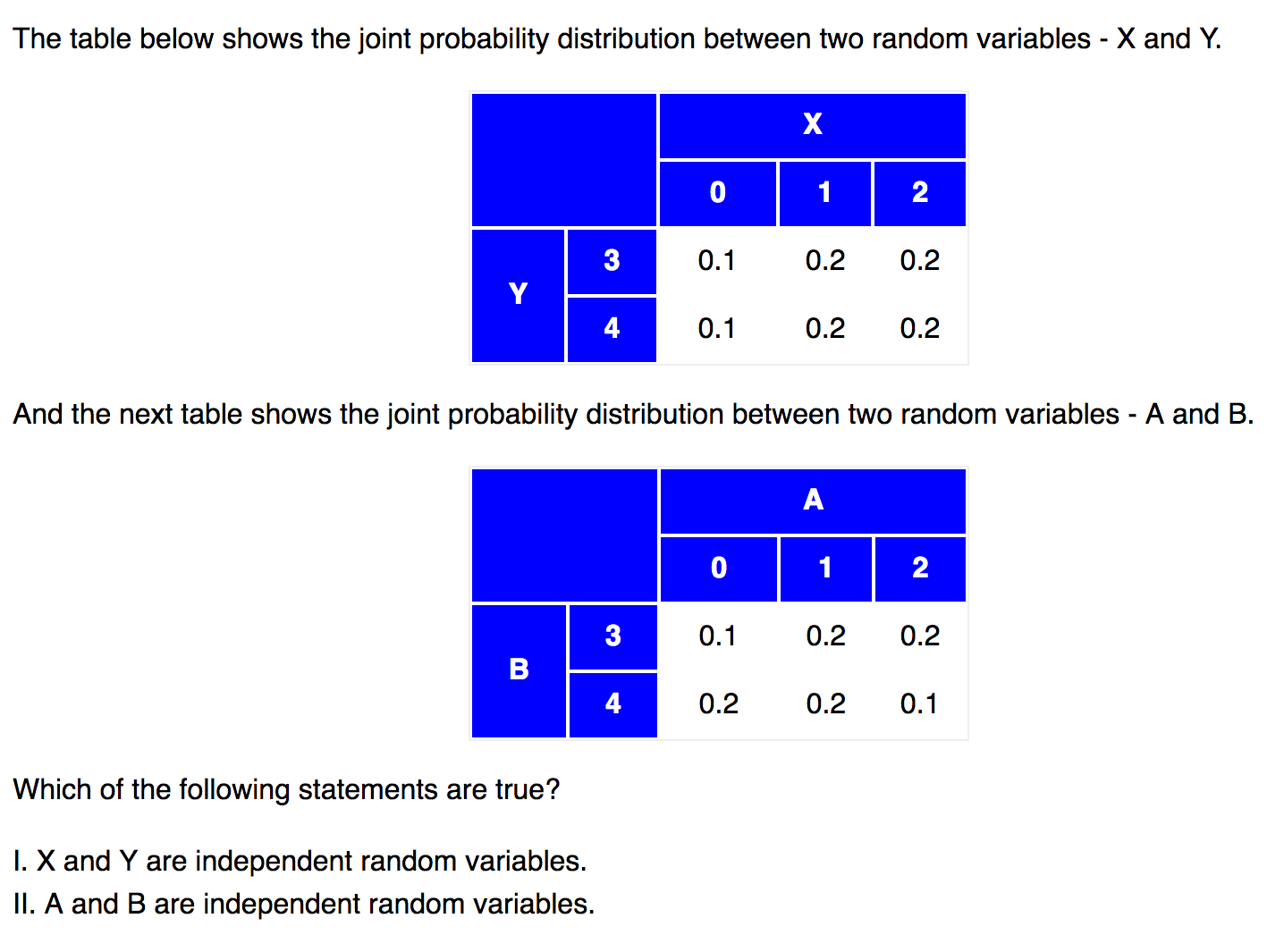
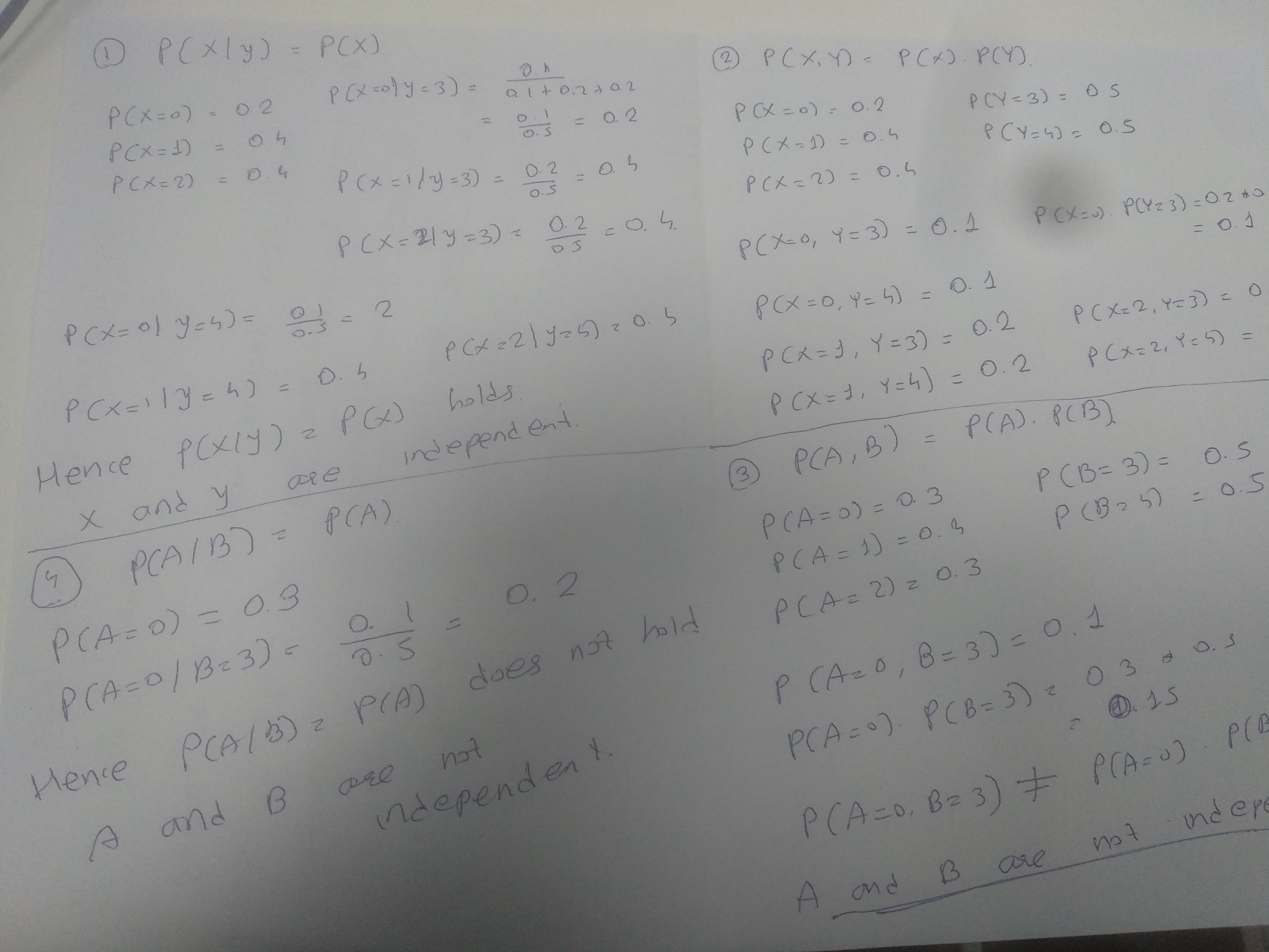
If two random variables, X and Y, are independent, they satisfy the following conditions.
P(x|y) = P(x), for all values of X and Y.
P(X, Y) = P(x ∩ y) = P(x) * P(y), for all values of X and Y.
Here is an example from [6]. Ans is that X and Y are independent, A and B are not.
Margin is the distance between hyperplane and closest training data point
We want to select a hyperplane for which this distance is maximum
Once we identify optimal separating hyper plane there can be many equidistance training points with the shortest distance from hyperplane
Such point are called support vectors
These points support the hyperplane in a sense that if they are moved slightly optimal hyperplane will also move
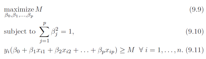
Training
Equation 9.10 ensures that left hand side of equation 9.11 gives perpendicular distance from the hyperplane
Equation assumes y has two values (+1) and (-1)
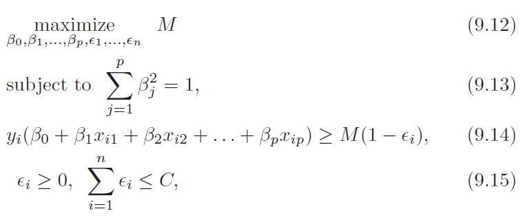
Support Vector classifier
Maximum margin classifier does not work when supporting hyperplane does not exist.
Support vector classifier relaxes optimization objective to get that work
Unlike maximum margin classifier this one is less prone to overfit as well
The formal one is very sensitive to change in single observation
Also know as soft margin classifier
ε variable allows training point to be on wrong side of margin
If ε > 0 it is on the wrong side of margin
If ε > 1 it is on the wrong side of hyperplane
Parameter C is the budget that constraints how many points are allowed on wrong side of hyperplane
C is selected with cross validation and controls bias variance trade off
Point that lies directly on the margin or on the wrong side of margin for their class are called support vectors
Because these points affects the choice of hyperplane
And this is the property which makes it robust to outliers
LDA calculates mean of all the observation
However LR is less sensitivity to outliers
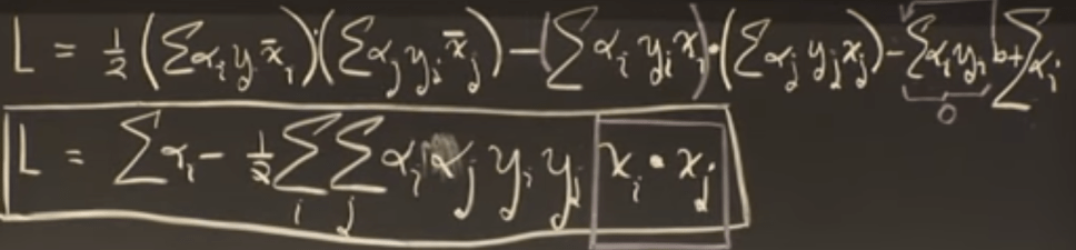
Computation note – when we try to solve above optimization problem with lagrange multiplier we found that it depends on dot product of training samples
This will be very important when we discuss support vector machine in next section
Dot product is only with support vector, both while training and while solving [1]
Support vector machine
Above two classifier does not work when desired decision boundary is not linear
One solution is to create polynomial features (as we generally do for LR)
But fundamental problem with this approach is that how many and which terms you should create
Also creating large number of feature raises computational problem
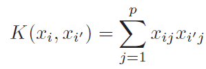
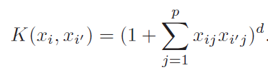
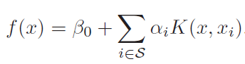
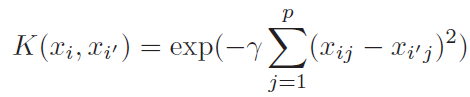
For the case of SVM, that fact that it involved only dot product of observation allows us to perform kernel trick.
Kernel acts as similarity function
Above equation makes it clear that we are not calculating(and storing) higher order polynomial still taking the advantage of it
Second one is polynomial kernel and last one is radial kernel
LDA models probability with multivariate Gaussian function
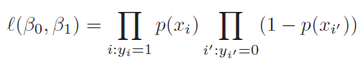
LR find maximum likelihood solution
LDA find maximum a posterior using Bayes’ formula
When classes are well separated
When the classes are well-separated, the parameter estimates for logistic regression are surprisingly unstable. Coefficients may go to infinity. LDA doesn’t suffer from this problem.
LR gets unstable in the case of perfect separation
If there are covariate values that can predict the binary outcome perfectly then the algorithm of logistic regression, i.e. Fisher scoring, does not even converge.
If you are using R or SAS you will get a warning that probabilities of zero and one were computed and that the algorithm has crashed.
This is the extreme case of perfect separation but even if the data are only separated to a great degree and not perfectly, the maximum likelihood estimator might not exist and even if it does exist, the estimates are not reliable.
The resulting fit is not good at all.
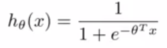
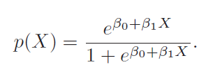
Math behind LR
For example suppose y = 0 for x=0 and y=1 for x = 1. To maximize the likelihood of the observed data, the “S”-shaped logistic regression curve has to model h(Θ) as 0 and 1. This will lead β to reach infinite, which causes the instability.
Few terms:
Complete Separation – when x completely predicts both zero and 1
Quasi-Complete separation – when x completely predicts either 0 or 1
When can LDA fail
It can fail if either the between or within covariance matrix(Sigma) is singular but that is a rather rareinstance.
In fact, If there is complete or quasi-complete separation then all the better because the discriminant is more likely to be successful.
LDA is popular when we have more than two response classes, because it also provides low-dimensional views of the data.
In the post on LDA, QDA we had said that LDA is generalization of Fisher’s discriminant analysis (which involves project data on lower dimension to that achieves maximum separation).
LDA may result in information loss
The low-dimensional representation has a problem that it can result in loss of information. This is less of a problem when the data are linearly separable but if they are not the loss of information might be substantial and the classifier will perform poorly
Another assumption of LDA that it assumes equal covariance matrix for all classes, in which case we might go for QDA. Blog post on LDA, QDA list more consideration about the same.
{In practice it is used more for classification than for regression}
This resemble gaussian mixture models in that you git one gaussian for each class.
Don't forget one important difference though. LDA is supervised, Mixture models are unsupervised.
Linear Discriminant Analysis (LDA)
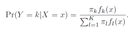
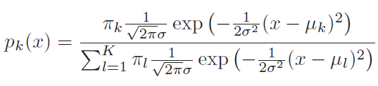
In logistic regression (LR), we estimate the posterior probability directly. In LDA we estimate likelihood and then use Bayes theorem. Calculating posterior using bayes theorem is easy in case of classification because hypothesis space is limited.
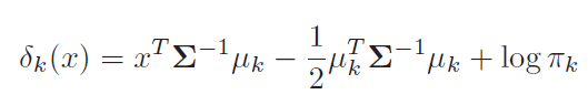
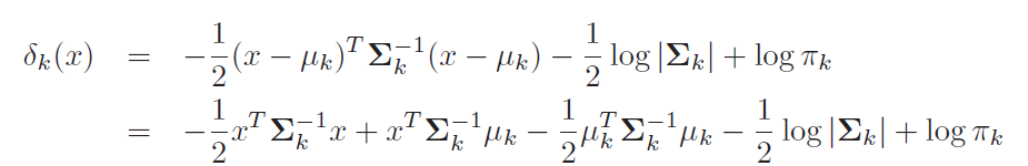
Equation 2 computes probability of class k given x. This is a posterior instead of just point estimates.
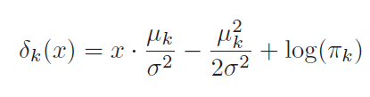
Equation 4 is derived from equation 3 only. Probability(k) would be highest for the class for which Delta(k) will be highest.
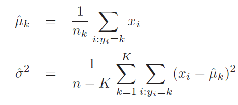
LDA estimates mean and variance from data and uses equation 4 for classification.
We also need to estimate π_k, which I think would be n_k/N.
Assumptions made:
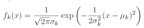
f(x) is normal
Variance(sigma) is same for all classes
When more than one predictor, we go for multivariate gaussian
Some comparisons
Compare this with mixture models, where there is a responsibility vector for each sample
There labels are not available (unsupervised learning) and hence is solved by EM (Expectation Maximization)
Compare this with naive bayes, there assumption is each feature is independent
Here we have parameter for each (class, feature), there we have parameter for each feature
Also here f captures probability of class (k) given x, there after bayes rules we calculate probability of x given class k
Hence the name naive bayes
Here we have joint distribution (multivariate gaussian, there it is independent distribution for each features)
Both LDA and navie bayes try to calculate posterior while logistic regression maximizes likelihood function
Quadratic Descriminant Analysis (QDA)
Unlike LDA, QDA assumes that each class has its own covariance matrix. It is called quadratic because below function is quadratic of x.
When to use LDA, QDA
This is related to bias variance trade-off
For p predict and k classes
LDA estimates k*p parameters
QDA estimates additional k*p*(p+1)/2 parameters
So LDA has much lower variance and classifier built can suffer from high bias
LDA should be used when number of training sample are less, because we want to avoid high variance problem
QDA has high variance, so it should be used when number of training samples are more
Another scenario would the case when common covariance matrix among K classes is untenable
A note on Fisher’s Linear Discriminant Analysis
It is simply LDA in case of two classes.
We can derive this similarity mathematically.
In literature we found it from the perspective that it project data on a line which achieves maximum separation
We can state without loss of generality that LDA also provides low dimensional view on data
Math
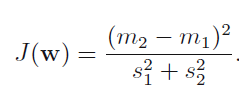
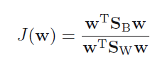
We want to project 2-D data on a line which
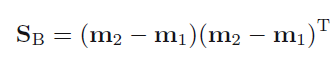
maximizes the difference between projected mean
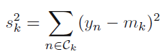
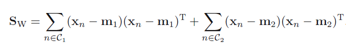
minimizes within class variance
Such a direction can be found by maximizing fisher criterion (J)