[Paper] RankNet to LambdaRank to LambdaMART

Microsoft had published a paper on RankNet in 2005, which also won ICML’s test of time award in 2015. Subsequent improvement to that algorithm were lambdaRank and lambdaMART. The later had also won 2010 – learning to rank challenge. Current paper[1] summaries all three algorithms and incremental improvement they are mapping. It is written by Chris Burges who was involved in these development since RankNet.

Quick Gist

  • RankNet was trained using Neural Net.
  • RankNet was trained to minimize pair-wise differences.
  • LambdaNet was designed to maximise NDCG.
    • Which is more relevant to IR compared to pair-wise differences.
  • LambdaMART started using tree based boosting algorithms (MART, XgBoost etc)

RankNet

  • For a given query (q), we have two items (i and j)
    • I am writing down item but it would be any document (web page for example)
    • We will have features for
      • query
      • item
      • query item pairs
  • For both (q, i) and (q, j) we pass them through NeuralNet and get scores -> si and sj
    • We will also pass pairs which has same supervised label
  • We need to decided a loss function based on si and sj, gradient of which we will back propagate.
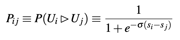
  • Computed probability formula y_hat
  • Supervised probability label y = (P_ij_bar) = (1 + S_ij) / 2
    • S_ij = { 0, 1, -1}
      • 1 if ( i is more relevant then j)
      • 0 if (i is less relevant then j)
      • 1/2 if both have same relevant scores
    • y will be in {0, 1/2, 1}
  • sigma determines shape of sigmoid
    • We would go to difference of (si – sj) on x-axis and read corresponding value from y axis.
    • sigma determines steepness around 0
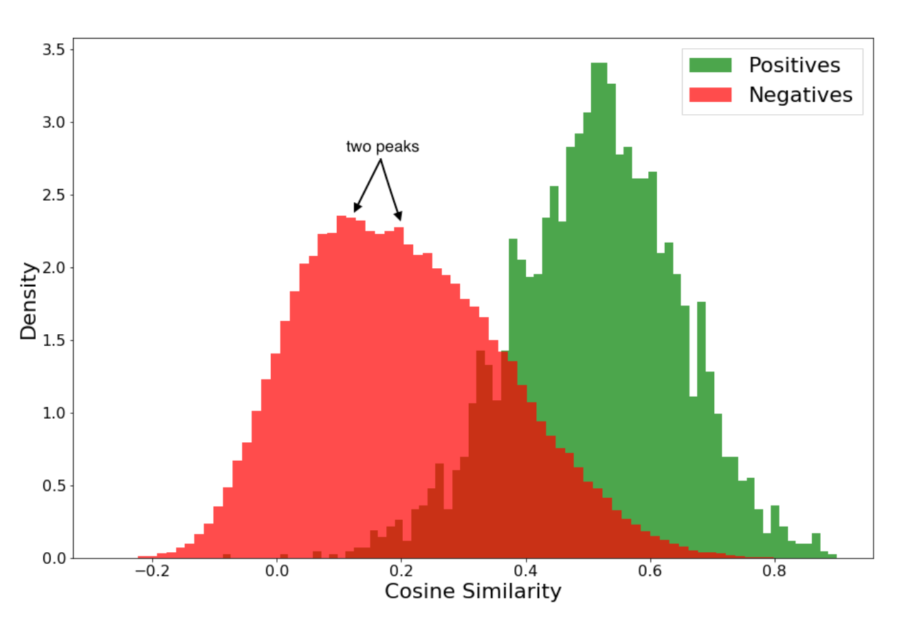
    • This technique is known as temperature scaling. In tower network people use is when passing cosine similarity value to sigmoid.
    • Technique is useful when input has limited range
      • Cosine similarity has range (-1, 1)
      • s_i – s_j would also have smaller range
  • Cost function is cross entropy
  • One observation here is that when si = sj
    • cost = log 2 > 0
    • Document with different label but same score are still pushed aways from each other.

Speeding up RankNet Training by factoring

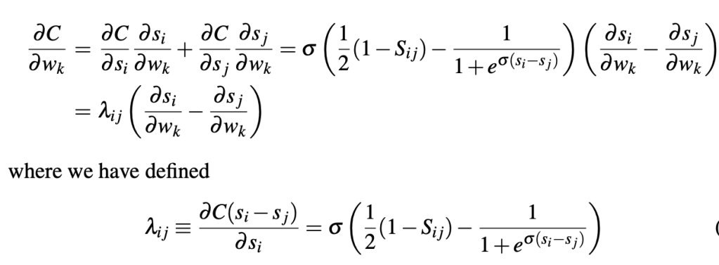
Defining lambda_ij

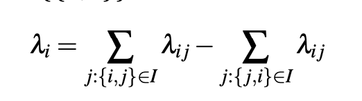
Defining lambda_i

  • What speedup did we achieve
    • Earlier for a given query we were computing lambda_ij for each pair and updating weights
    • Now we are computing lambda_i for each document and then update weight for given query
      • You can correlate this to going from SGD to mini-batch
      • We can do SGD at query, pair level or query level. We choose later.
  • Intuition of lambda_i
    • Direction(+Ve/-Ve) and magnitude where we want document to move
      • Move up/down in the ranking

LambdaRank

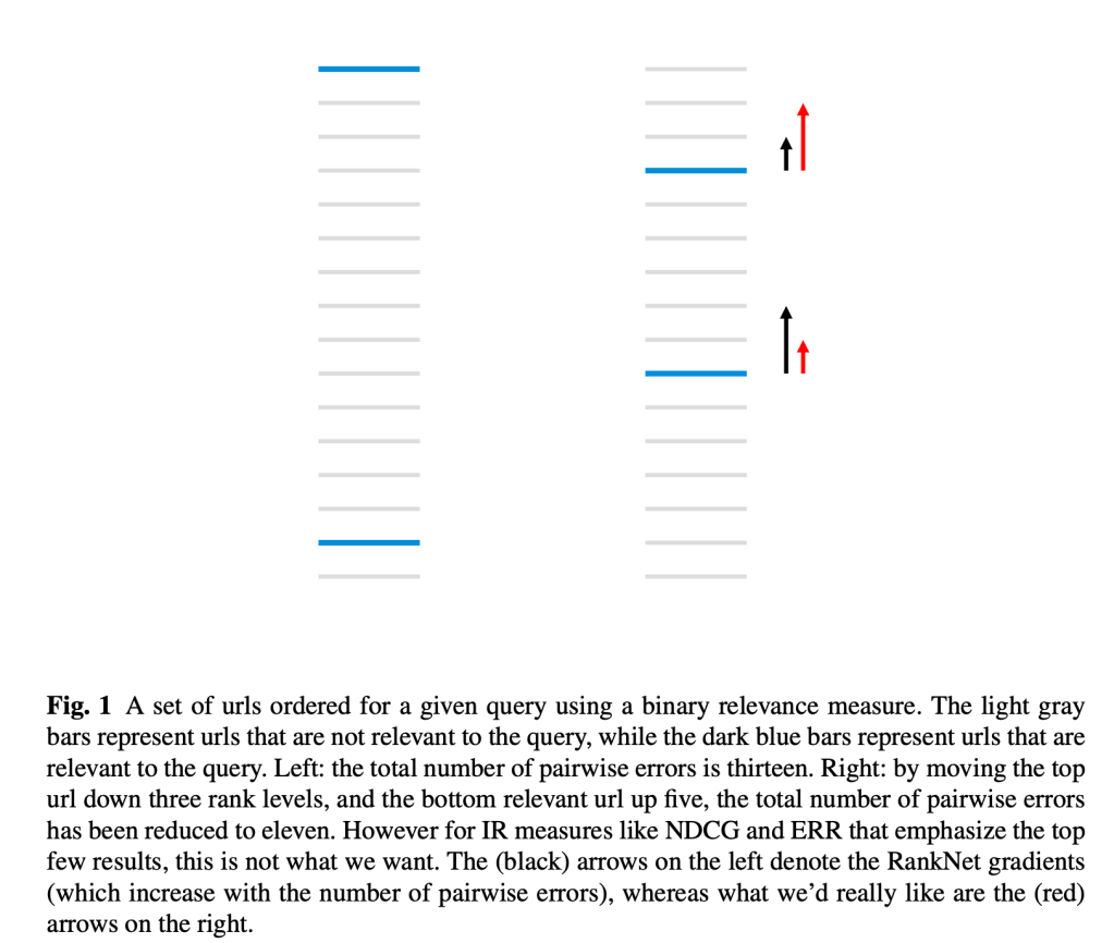
Figure below and caption explains why reducing pairwise difference does not necessarily results in increase of IR metrics. And LambdaRank is a way to optimize for IR metrics faster.

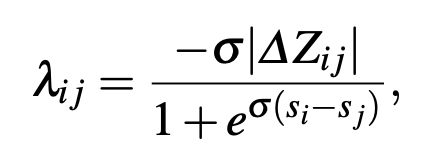
LamdaRank modified lamda_ij equation empirically as follows and it seemed to work well. We could do this because we don’t need to know actual cost function as long as we compute lamda_ij and then lamda_i

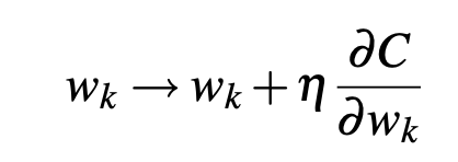
This becomes maximisation problem so we move in direction of gradient.

LambdaMART

  • MART – Multiple Additive Regression. Trees. For more info read the post on gradient boosting
  • To work with MART we need to specify two things
    • Gradient of loss function, which will be used to fit the trees
    • For the region in tree compute leaf value, that is done using line search/newton’s method
  • We had empirically defined lambda as gradient in lambdaRank, we use same lambda as gradient here as well.
  • For above lambda gradient, paper defines empirical cost function and then derives value at leaf nodes using newton’s method.
  • Key difference to observe between lambdaRank and lambdaMART
    • Lambda rank updates all weights (of classifier) after each query is examined
    • Leaf value at lambdaMART is computed for all query, item pairs that falls into that leaf
      • This allows lambdaMART to update splits and leaf values such that it may decrease utility for some queries but overall utility increases.

Reference

[0] : https://www.microsoft.com/en-us/research/blog/ranknet-a-ranking-retrospective/

[1] : https://www.microsoft.com/en-us/research/uploads/prod/2016/02/MSR-TR-2010-82.pdf

On Interleaving

This post summarises some concepts around interleaving. Take away for me in the topic is realisation that in some cases interleaving can be conclusive while a/b test is not. (examples of search improvement on small % of queries) and the intuition that why it converges faster. Also there is a broader topic – design of experiments. It is generally used in search systems and recommender systems. Both can come under umbrella of retrieval systems.

What is interleaving ?

  • It is a method to evaluate ranking system.
  • If we want to measure effectiveness of two ranker, we prepare a merged list and observe customer’s interaction on that.

Why do we need interleaving ?

  • It allows us to experiment faster.
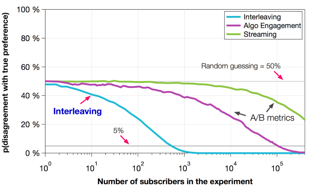
    • It converges faster than a/b tests
  • For search systems many times a/b test might not converge at all
    • Say an improvement is affecting small % of search queries
  • Search system has low convergence say 4 %. How to measure algorithm that improves 0.5 % on top of that.
    • Lots of impressions are needed for convergence in a/b test.

Illustrative Examples

  • Shoe
    • Suppose for a given shoe design we have two compelling soles, we want to measure which one has better resistance to wear/tear
    • We have 100 people to test on
    • option 1 – classic a/b test
      • 50 people get each type of shoes
      • Two variability
        • How active the person under tests it
        • Quality of sole
    • option 2 – interleaved test
      • Different sole in left and right pair of shoe
      • Just one variability
        • Quality of sole
  • Soda [0]
    • We want to test what is more popular among population – Pepsi or Coke ?
    • option 1 – classic a/b test
      • Split population into two groups
        • One group receives Pepsi
        • Another one receives Coke
      • Measure soda consumption between two
      • Variability
        • Wide variation in soda consumption habit
        • Heavy soda consumer would be small % of population but large % of contributor
    • option 2 – interleaving
      • Allow people to choose either Pepsi or Coke.
      • Don’t mark a label, but can be visually distinguishable

For some tests interleaving is not possible.

  • In the shoe examples instead of sole, if we have two different design of shoe
  • In search systems, if you are changing some UI elements

Two tests Netflix did while introducing new interleaving system

  1. Compare sensitivity against traditional a/b tests [0]
    1. Before the test it was known that algorithm B is better than A
    2. They measure no of impressions it took to converge

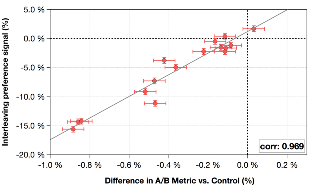
2. Correlation of interleaving result with a/b tests [0]

On Metrics

  • Search systems have business metric like conversion & revenue
  • Netflix has business metrics like retention and streaming hours

Reference

[0] Netflix blog

[Paper] Semantic Product Search

  • Paper is related to search systems for e-commerce.
  • Shortcoming of BM-25
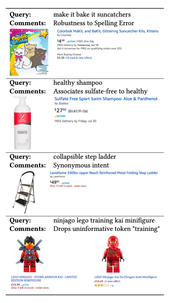
    • lack of understanding of hypernyms, synonyms, antonyms
      • hypernym – general/broad word
      • Color is hypernym for red
      • Examples
        • Red dress and burgundy dress
        • sneakers and running shoes
    • Morphological variants (woman vs women)
      • Stemming and lemmatization is typical solution
      • Requires numerous hand-crafted rules
        • Converts reading glasses to reading glass
    • Sensitivity to spelling error
      • Typically solved by spell correction algorithms

Architecture

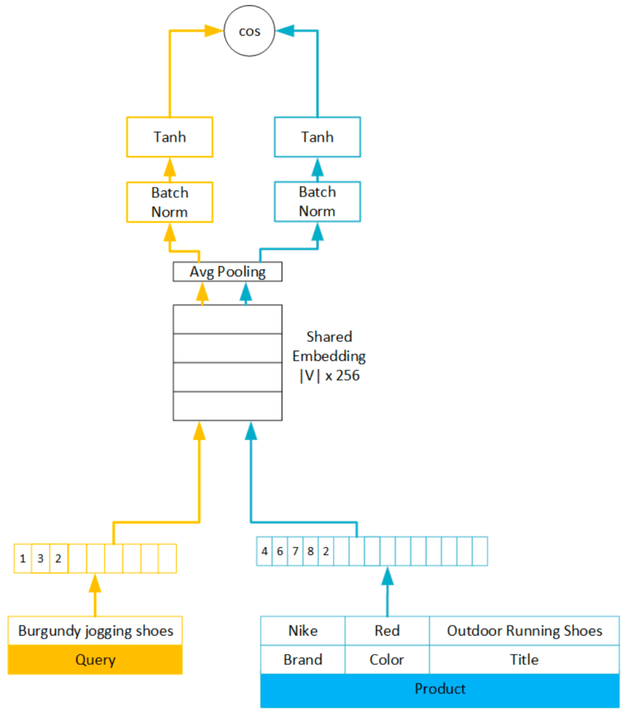
  • Sharing embedding layer in siamese network work well, capturing local word level matching even before training this network.
  • Average pooling
    • Comparing to LSTM performance of average pooling reduced by just 0.5 %
    • Evaluation metric were MAP and Recall@100
    • It helped computationally
    • Unlike web search query and items titles have smaller length
    • Query also does not have stop words
  • Batch Normalisation
    • Length of items are generally longer than query
    • They had observed difference in magnitude after avg pooling of query and item
    • I have seen people using FC layer instead to have separate parameters

Loss Function

  • They first tried with 2 part hinge loss
  • Analysing the overlap items they found that they were clicked but not purchased.
    • They note that from matching standpoint these products are okay to show to customer
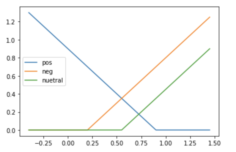
  • So they introduced third term and decided it’s threshold to be 0
  • EmpIrical values used episolon (+) = 0.9, episilon (-) = 0.2
  • My view on this
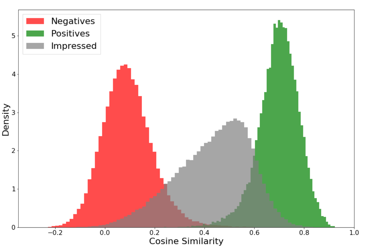
    • For the products that has clicks but not orders, new loss tries to keep it below 0.55
    • 2 part hinge loss was for purchased vs random items
    • Some of those random items had got clicks
    • For positive items when we get similarity above 0.9 it should contribute 0 to loss
    • For negative items if we get similarity below 0.2 it should contribute 0 to loss
    • For neutral items if we get similarity below 0.55 it should contribute 0 to loss
  • y_hat is cosine similarity
    • Based on which loss is calculated
    • Instead of passing cosine similarity to sigmoid they are passing it through hinge function.

Tokenization Methods

  • Word unigram
  • word n-gram
    • To preserve information about word ordering
    • They preferred word n-gram over LSTM or CNN
  • Character trigram
    • Robust typos (iphone & iphonr)
    • Compound words (amazontv & firetvstick)
    • Item parts and sizes
      • Tires have different sizes
      • TVs have different model
  • Handling unseen words
    • Common NLP techniques
      • Mask the input
      • use same embedding for all unseen words
    • What they choose
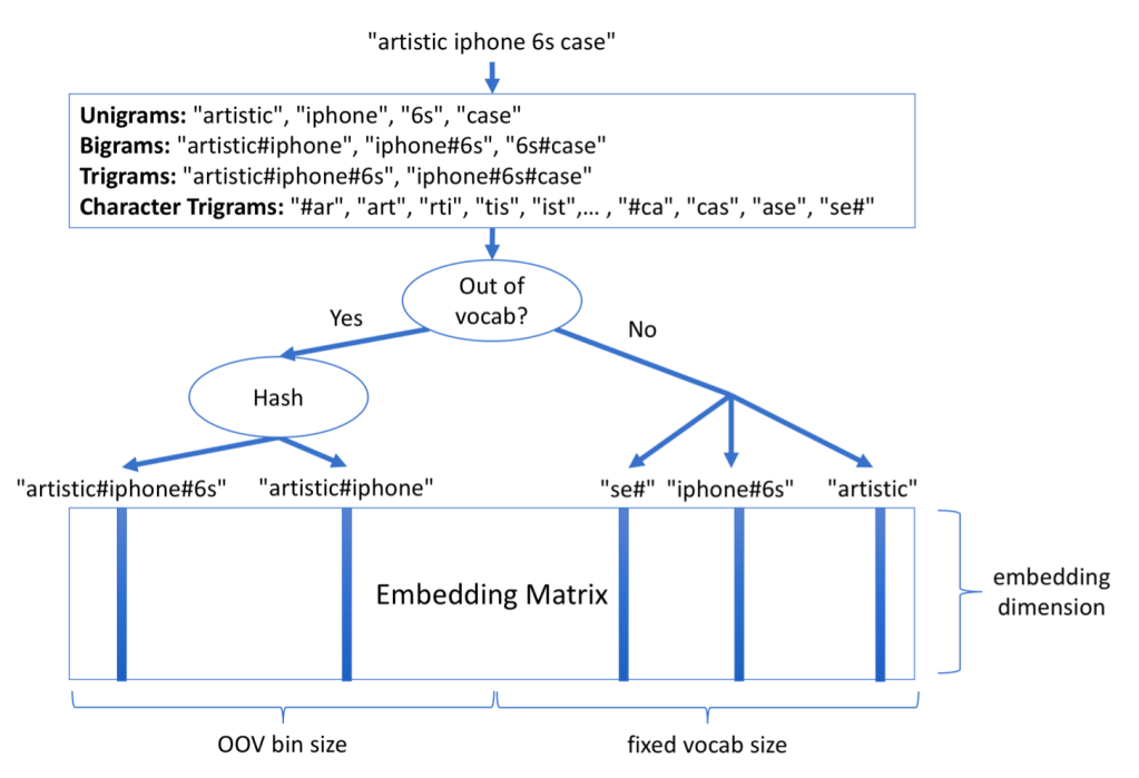
      • Keep more embedding space for unseen words
      • Hash them to get the bucket
    • Enough space is allocated for frequent words and they are not hashed
      • 10k or 100k of n-grams are kept
  • Combining tokenization
    • One approach
      • Separate embedding for unigram, biagram and character trigrams
      • Compute. weighted sum of cosine similarity individually
    • Their approach
      • Consider them as bag or words

Data

  • Time range
    • Training data – 11 month
    • Eval data – 1 month
  • Trick of aggregating count as weight
    • Weight while computing the loss, simple multiplication ( I had done that in synonyms as well )
    • 54 billion query product training pairs
    • Reduced to 650 million
  • Ratio
    • 1 purchased
    • 6 impressed
    • 7 random
    • They plan for both matching and ranking
    • Matching -> Differentiate between (purchased + impressed) from random
    • Ranking -> Differentiate between purchased and impressed
  • Query Preprocessing
    • Changes queries to list of token IDs
    • array length = 99 % tile of query token length
    • Smaller tokens are padded to right
  • Item preprocessing
    • One approach
      • Embed every attribute independently and concat
    • Their approach
      • Ordered Bag of words for title and attributes
      • Issue was variability in attributes and lack of structured data across items

Model Evaluations

Evaluation Metrics

  • Matching
    • Recall@100 and MAP
      • Used for tuning model hyper parameter as well
    • 20k queries and sub-corpus for those queries
      • Around 1M items
      • Ordered + Impressed + Random
  • Ranking
    • NDCG and MRR
    • Purchased + Impressed

Evaluation Results

  • Table 1
    • L2 variant of hinge loss outperforms L1
      • They hypothesise that L2 is more robust to outliers
    • 3 part hinge loss outperforms 2 part in matching but not in ranking
      • Introduction of 3rd part forced purchased and random to be more separated
  • Table 2
    • LSTM, GRU vs avg Pooling for aggregation
      • Comparison is made for various losses
      • Average pooling is performing similar or slightly better
        • Definitely reduces computation time
      • Since query and product title are relatively short this works well
      • Recurrent methods are expressive but introduces specialisation between query and title
        • Some may argue it is a good thing
        • They argue that it might not capture local word level mapping
  • Table 3
    • Compares different tokenization methods
    • Vocab sizes in embedding space
      • 125k – unigram
      • 25k – bigram
      • 64k – character trigram
      • 500k – Out of vocabulary (OOV) bins
    • Advantage of adding bigrams
      • Example – Chocolate milk vs milk chocolate
    • Advantage of character trigrams
      • Robustness to spelling error
    • OOV adds additional parameters
      • case 1 : 500k unigrams
      • case 2 : 125k unigrams and 375k OOV
      • case 2 performs better
  • Table 4
    • Batch vs layer vs no normalisation
    • query sorted data vs shuffled data
    • Optimum combination was using batch normalisation with shuffled data
    • Query sorted data did not have much effect on layer normalisation but was on batch normalisation
      • Batch estimates for mean and variant would be biased for batch normalisation
  • Table 5

Online evaluations

  • Three categories
    • toys and games, kitchen and pets
  • Conversion rate, revenue and other KPI increased with statistical significance
  • Challenges
    • Precision was decreased
    • To mitigate they added guardrails using some heuristic and ranking models to filter non relevant items
    • Not that recall@100 was metric for matching task and not precision.

Training Acceleration

  • Increasing query product pairs from 200 million to 1.2 billion had improved matching metric by 10 %
  • Data parallel training
    • Idea
      • Split data
      • Same model on multiple GPUs
      • Take the average of gradient in the end
    • Cons for this architecture
      • Limits embedding metric
        • It has to fit on single GPU
      • Data parallel approach has high communication overhead
        • We need to weight till forward pass from each GPU is available
  • Model parallel training
    • Pros in this architecture
      • Simplicity of average pooling
      • Siamese has some parallelism by default
    • How they implemented
      • Embedding metric is split across GPUs, across embedding dimension
        • Hence we need to concat to get final embedding vector for each token
          • Concatenation requires O(2k) communication of floating point numbers
        • Partial token embeddings are averaged at each GPUs
      • Full dataset is sent to all GPUs
  • In the result section they have told that embedding dimension was 256
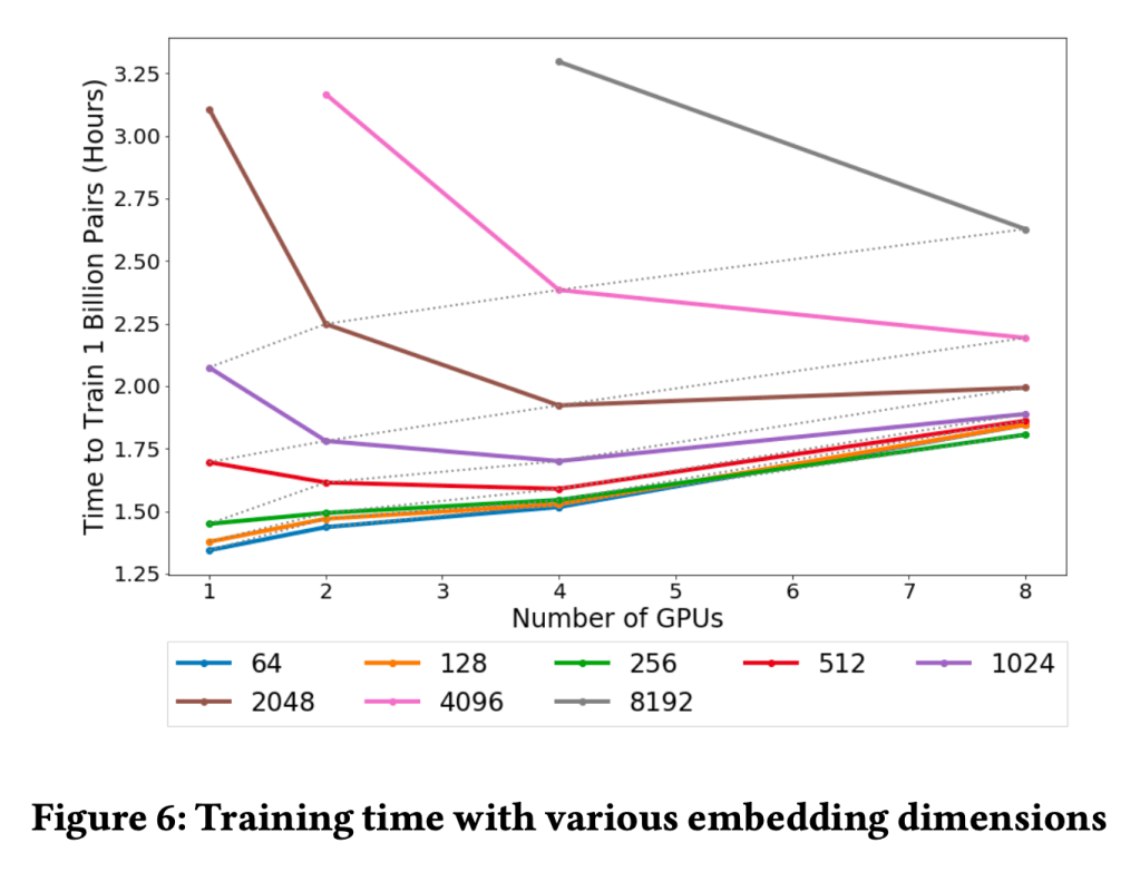
  • Explaining above image
    • For low embedding dimension time-to-train increases with number of GPUs but for high embedding dimension time-to-train decreases with number of GPUs
    • Dotted line
      • Following two should have same training time
        • 2048 embedding with 1 GPU
        • 1024 embedding with 2 GPU
      • Doted line is for the ration of embedding_size/GPU
      • With ideal scaling it would be horizontal

Exampels

Quantile Function (Inverse CDF)

Introduction

CDF maps input between in [0,1]. That is CDF(x) -> (0,1)

Quantile function takes input in (0,1) and return x.

  • Not all functionals are invertible.
  • Continuous distribution easily satisfies this property
  • For discrete distributions we take innfimum of all values [0]

Application in Sampling

  • Suppose we want to sample from a given distribution
  • We can make a quantile function of it
  • Sample uniformly from [0,1], call it p
  • x = quatile(p)
  • x is the sampled value [1]

Application in point estimation

  • Suppose you want to model CTR (click through rate)
  • CTR lies in (0,1) and can be presented via beta distribution
  • You have clicks and impressions for two ads/items anything
  • We are more confident about CTR when you have more impressions
  • We can construct a beta distribution with mean as point CTR.
    • ctr = beta(clicks, impression-clicks)
    • Recall in thompson sampling we were increasing alpha and beta by 1
  • Now we take 1%, 5%, 10% from quantile function.
    • We would generally have features for historical clicks and impressions.
    • If we have CTR as a feature, we can have this 5% number instead of a point estimate.
  • When we have more impressions ctr_x would be close to mean ctr (point estimate), else it will be less
  • On side node – this way of constructing distribution gets us away from point estimation and can be used in bayesian approaches

Reference

[0] https://stats.stackexchange.com/questions/212813/help-me-understand-the-quantile-inverse-cdf-function

[1] https://stats.stackexchange.com/questions/184325/how-does-the-inverse-transform-method-work/184337#184337

Probabilistic Clustering

This post serves as a lecture summary of a course offered by the University of Washington, which can be accessed at the following link: University of Washington – ML: Clustering and Retrieval.

Sample code related to the course can be found on GitHub at: Sample Code for EM Algorithm.

In this lecture, we will cover several important topics:

  1. Why we need probabilistic clustering: We will explore the motivations behind using probabilistic clustering methods, which allow for soft assignments to clusters rather than rigid assignments.
  2. Mixture models: We will dive into the concept of mixture models, which are a probabilistic approach to clustering. Mixture models allow data points to belong to multiple clusters with different probabilities.
  3. Expectation Maximization (EM): We will study the Expectation Maximization algorithm, a powerful iterative algorithm used to estimate the parameters of mixture models. EM alternates between the expectation step, where cluster assignments are updated based on current parameter estimates, and the maximization step, where the parameters are updated based on current cluster assignments.

Why we need probabilistic clustering ?

To understand the need for probabilistic clustering, let’s consider the problem of determining user preferences based on their feedback. Suppose users provide feedback on whether they liked or disliked an article. We want to gather this feedback and group it into clusters to gain insights into their preferences.

For instance, imagine a user who likes an article about the first human landing on Mars. This article could be relevant to both world news and science news categories. In such cases, assigning articles to clusters with a hard assignment (where an article belongs to only one cluster) may not capture the complete picture. Soft assignment to clusters, where an article can belong to multiple clusters with different probabilities, is more suitable.

Now, let’s explore some scenarios where the traditional K-means algorithm fails:

  1. Clusters with Different Spreads: When clusters have varying spreads, simply deciding based on a single sample may not provide an accurate representation. Instead, it is important to consider the number of data points within each cluster. Assigning an ambiguous point to a cluster that has more data points can be a more meaningful approach.
  2. Overlapping Clusters: In cases where clusters overlap, soft assignment becomes crucial. It allows for assigning data points to multiple clusters based on the degree of membership.
  3. Clusters with Different Shapes or Orientations: When clusters have distinct shapes or orientations, measuring the distance to the cluster center alone is insufficient. Considering the shape of the clusters is necessary for accurate clustering.

One approach to address these challenges is using K-means with scaled Euclidean distance. This modification results in clusters represented by axis-aligned ellipses, accommodating different spreads in each dimension. However, determining appropriate weights for each dimension in the calculation remains a question that needs to be addressed. Shape is still axis-aligned ellipses, which is a limitation in itself.

Motivating application

Let’s consider the task of clustering images based on their color composition. One approach is to compute the average values of the red (R), green (G), and blue (B) channels for each image. This results in representing each image as a single 3-dimensional vector [R, G, B], capturing the average color values.

By applying clustering algorithms to these image vectors, we can group similar images together based on their dominant color characteristics. Although our data is unlabeled, we can observe potential clusters such as:

  1. Sky Cluster (Blue Dominated): Images that predominantly contain blue colors, such as those depicting clear skies, can be grouped into this cluster.
  2. Sunset Cluster (Red Dominated): Images showcasing vibrant sunsets with warm hues and red tones can be grouped into this cluster.
  3. Forest Cluster (Green Dominated): Images featuring lush green forests, landscapes, or vegetation will likely be grouped into this cluster due to their dominant green color composition.

Mixture Models

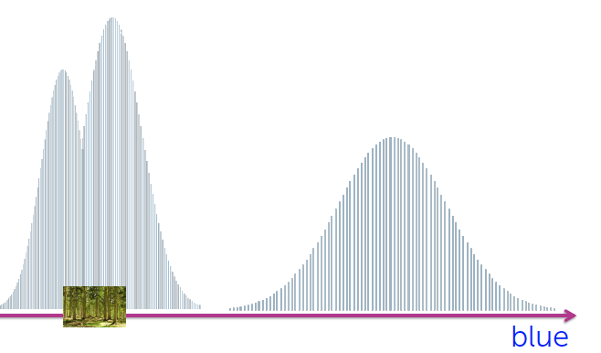
  • Here is how distribution of blue might look for all images
blue

We can model image clustering using a mixture of Gaussian distributions. The model consists of three Gaussian components, each with its own parameters (μ and σ). The final distribution is a convex combination of these components: π1g1 + π2g2 + π3*g3, where 0 ≤ π ≤ 1 and the sum of all π values is equal to 1.

Each mixture component represents a unique cluster, characterized by its own set of parameters (πk, μk, σk). In the case of multidimensional data, such as image vectors, each individual distribution is a multivariate Gaussian distribution.

Without examining the image vector, we can determine the probability of it belonging to cluster k using the πk value. Given an image vector x, we can estimate the probability of it belonging to cluster k as P(x | params) = P(x | μk, Σk), where Σ represents the covariance matrix in the multivariate Gaussian.

Clustering with soft assignment involves calculating a responsibility vector for each data point. The length of the responsibility vector corresponds to the number of clusters, which in this case is three (sky, forest, sunset). Each element of the responsibility vector represents the probability of a data point belonging to a specific cluster.

In the case of document clustering, where the dimensionality is high (proportional to the number of words in a vocabulary), keeping track of parameters for each Gaussian becomes computationally expensive. To address this, we simplify the model by considering only diagonal values in the covariance matrix, effectively restricting the model to axis-aligned ellipses. This approach is similar to K-means with scaled Euclidean distance, which also allows for axis-aligned ellipses.

However, the advantage of the mixture model is twofold:

  1. We do not need to specify weights for each dimension in advance; the model learns them from the data.
  2. Different clusters can have varying weights for each dimension, allowing for more flexible modeling of the data.

EM

Responsibility vector calculation with known cluster parameters

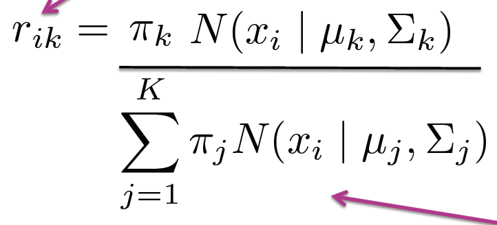
  • The responsibility vector can be calculated if we know the cluster parameters: π_k, μ_k, and ∑_k.
  • The responsibility vector is different from the π values.
  • Given a data point, we can find its corresponding responsibility vector by estimating the probabilities in that cluster.
  • The responsibility vector needs to be normalized after evaluating the probabilities.
a
  • This process is a consequence of Bayes’ rule.

Estimating cluster parameters with known responsibility vectors

  • It is similar to parameter estimation of a multivariate Gaussian.
  • Each data point, x_i, is multiplied, and there is no need to worry about the denominator since it is also not N (the number of data points).
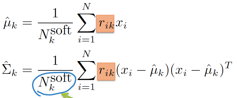
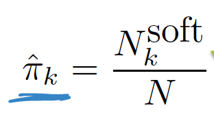
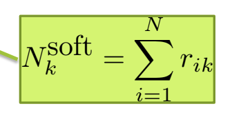
  • b1         b2      nk_soft
  • N_k_soft implies how many points belong to cluster 1
    • Also it is a soft assignment

EM Algorithm

  • E-step: Estimation of the responsibility vector given parameters.
  • M-step: Maximum likelihood estimation of the parameters given the responsibility vector.
  • These two steps are repeated until convergence.
  • The EM algorithm can be derived as a coordinate ascent algorithm and converges to a local mode.
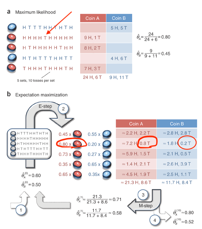
  • The biased coin example provides a good illustration of the EM algorithm. Check the image below

mj0nb

Challenges

  • The probability becomes infinite when the variance becomes zero.
  • This can occur when there is only one data point in a cluster, and the mean is itself with zero variance.
  • In high-dimensional spaces, this often happens, such as when a document does not have a specific word at all.
  • To solve this issue, a small value is added to the diagonal elements of the covariance matrix, similar to adding a prior in Bayesian approaches.

Relationship to K-means:

  • When a Gaussian has the same variance in all dimensions and shrinks to zero, the likelihood becomes either 0 or 1.
  • This behavior is similar to hard assignment, resembling the K-means algorithm.

Initialisation

  • Choose k observations at random and assign observations to nearest centroid
  • Above via k-means++
  • Solution of k-means
  • Grow mixture model by splitting cluster (sometime merging) until K clusters are formed

I have coded simple EM at [0]

References

[0] : https://github.com/arcarchit/datastories/blob/master/EM.ipynb

Thompson Sampling

Thompson sampling is one approach for Multi Armed Bandits problem and about the Exploration-Exploitation dilemma faced in reinforcement learning. It is also know as posterior sampling.

Challenge in solving such a problem is that we might end up fetching the same arm again and again. Bayesian approach helps us solving this dilemma by setting prior with somewhat high variance.

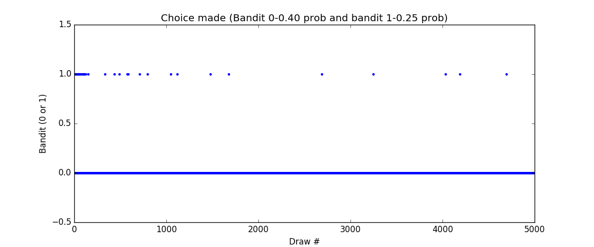
Here is the code for two armed bandit. One has success probability of 40% (bandit 0) and another has 25% (bandit 1).

We are using beta distribution for deciding which arm to pull. Beta distribution has two parameter alpha and beta. Higher values of alpha, pulls distribution towards 1. Beta distribution is always confined between 0 and 1.

How we train is that for each feedback we receive we increment alpha by 1 if it was success or beta by 1 in case of failure. For choosing the arm we draw random sample from the distribution of each arm and select the arm with highest value.

import numpy as np
import scipy.stats as stats
from matplotlib import pyplot as plt
class BetaThompson:
def __init__(self, num_bandits, prior_a, prior_b):
self.num_bandits = num_bandits
self.a = prior_a
self.b = prior_b
def learn(self, bandit, success):
if success:
self.a[bandit]+=1
else:
self.b[bandit]+=1
def suggest(self):
sampled_prob = []
for i in range(self.num_bandits):
dist = stats.beta(self.a[i], self.b[i])
prob=dist.rvs()
sampled_prob+=[prob]
return sampled_prob.index(max(sampled_prob))
class Gamble:
def __init__(self, num_bandits, binom_mean):
self.num_bandits=num_bandits
self.binom_mean=binom_mean
def gamble(self, bandit_no):
dist=stats.binom(n=1,p=self.binom_mean[bandit_no])
success = True if dist.rvs()>0.5 else False
return success
def main():
g = Gamble(2, [0.40, 0.25])
bot = BetaThompson(2, [1,1], [1,1])
choice=[]
for i in range(5000):
suggestion = bot.suggest()
result = g.gamble(suggestion)
bot.learn(suggestion, result)
choice+=[suggestion]
plt.figure(figsize=(12,5))
plt.plot(choice, 'b.')
plt.ylim([-0.5,1.5])
plt.title('Choice made (Bandit 0-0.40 prob and bandit 1-0.25 prob)')
plt.xlabel('Draw #')
plt.ylabel('Bandit (0 or 1)')
plt.savefig('choice.png')
if __name__== "__main__":
main()

And here is simulation results. We see that initially both the the armed are pulled frequently but slowly arm 1 is pulled less and less, but it is never straight away zero.

choice

Math Behind Increasing alpha and beta

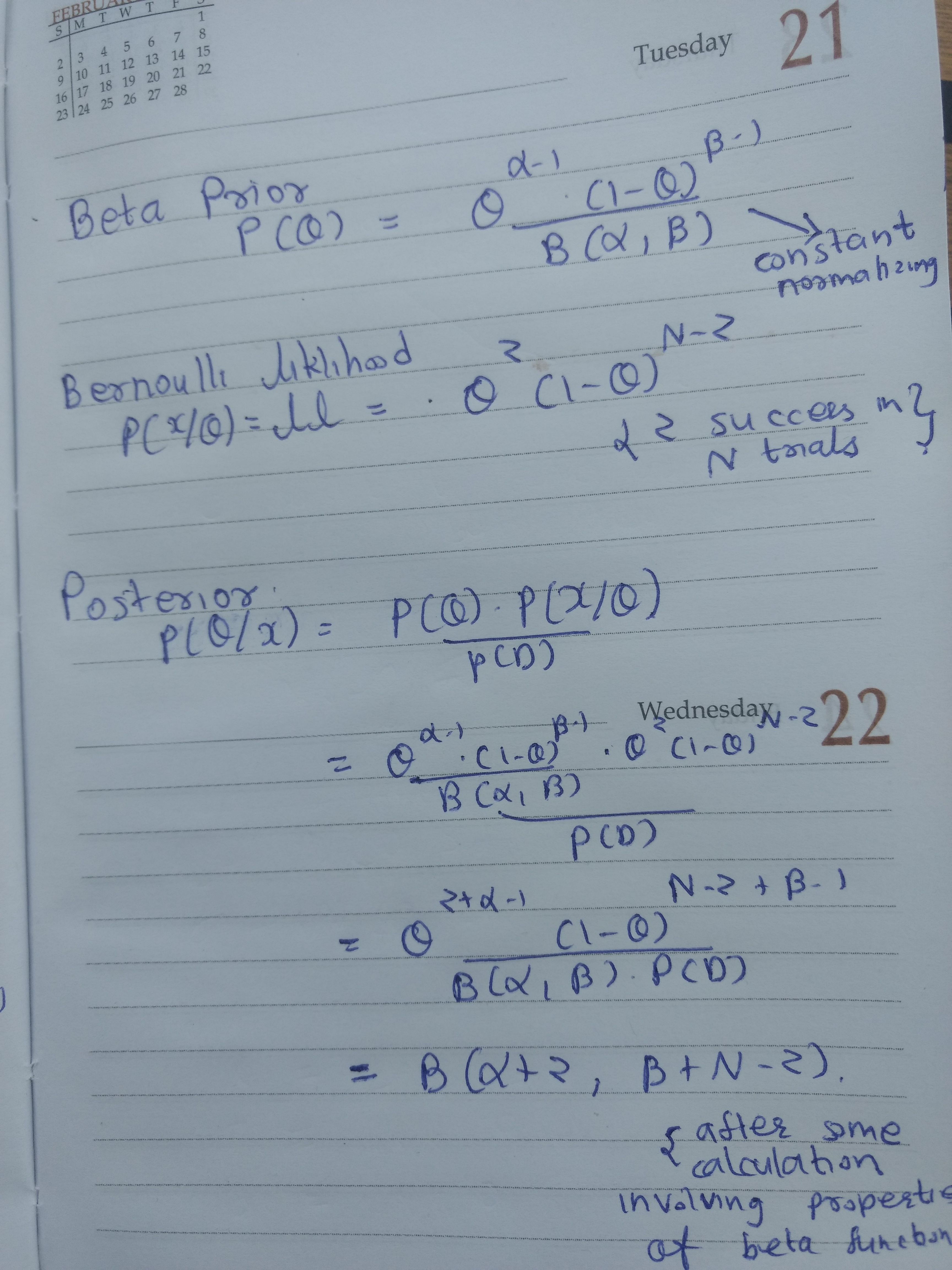
In one line posterior is beta distribution for beta prior and Bernoulli likelihood. In other words beta is a conjugate prior for Bernoulli likelihood. List of various conjugate prior is available at [1].

PDF of beta distribution is simple once you think in terms of the effect of alpha and beta.

Look at note below, formula of beta distribution is not complex, actually it is very similar to

bayesian

References

[1] : https://ocw.mit.edu/courses/mathematics/18-05-introduction-to-probability-and-statistics-spring-2014/readings/MIT18_05S14_Reading15a.pdf