Now let’s say we have 1000 words and 300 hidden units, we shall have 300,000 wights in both hidden and output unit, which are two many parameters.
Output label during training is one hot vector with 999 zeros and single 1. We randomly select 5 zeros and update weight for six words only. (5 zeros and single 1). The more frequent word is the highr the probability of it getting selected. Google paper has mentioned some emperical formula for this. This is know as negative sampling.
Above was for output layer. In hidden layer weights are updated only for input words. (Irrespective if it is negative sampling or not)
Training pair would be nearby words in predefined window
We can imagine how huge can that be
It is pair of words both one-hot encoded
Sure, we need to know previously size of our vocabulary (which will be dimension of one-hot vector)
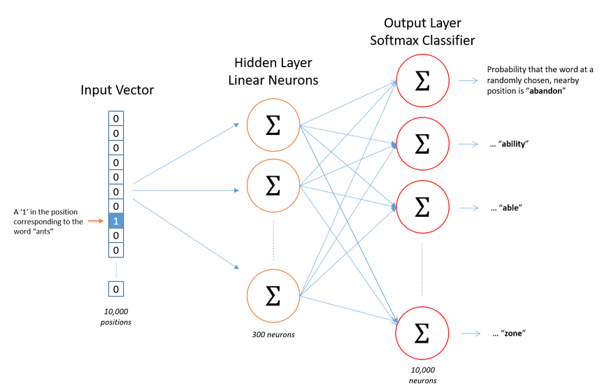
The paper google release was trained on google news data and used 300 dimension vector, which means 300 neuron in hidden unit. The paper lists this no and size of training words and efficiency.
Not there is one more parameter called named window size which was set to 5.
It means that 5 words before and after center words are considered as pair for training data.
There is no activation function on the hidden layer neurons, but the output neurons use softmax.
Why word2vec
Earlier NLP methods used to rely on synonyms/hypernyms which is not totally contextual
Earlier case was mainly one hot encoding of vector
“proficient” is synonym of good only in some context
New words are getting added everyday
All words are one-hot encoded
Somewhat similar word might be orthagonal
Size of vector become too large
Role of TF-IDF
It is a scoring mechanism
Instead of average vectors of all the words in document we can have weighted average by TF-IDF score
There are two more things:
Continuous Bag Of Words
Negative sampling
CBOW
It also takes average of context words
One argument in the favour that averaging is valid
Both CBOW and skip gram does not add non-linearity in hidden layer
Output layer uses softmax
Idea is that word-embedding is used to predict target word.
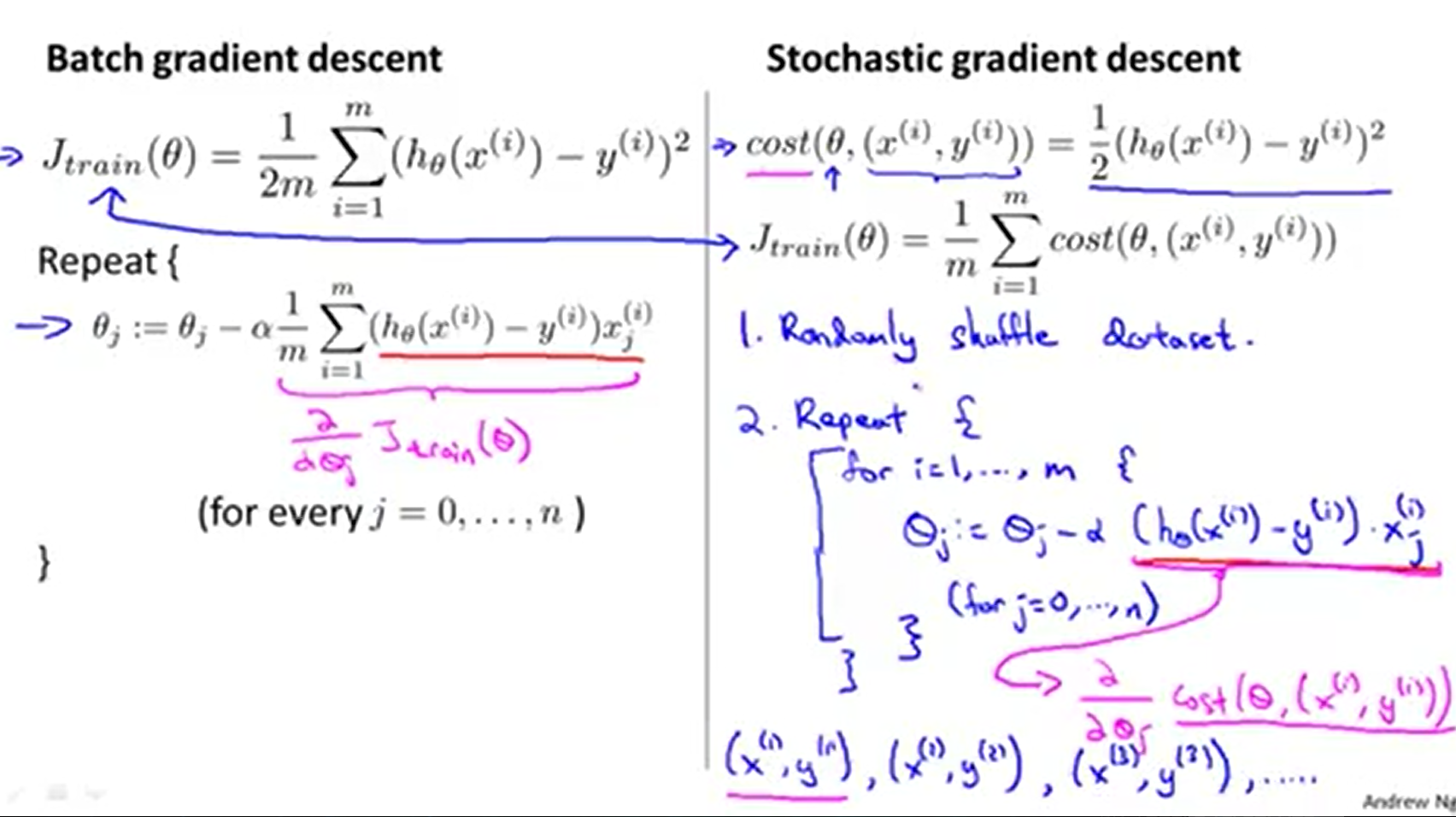
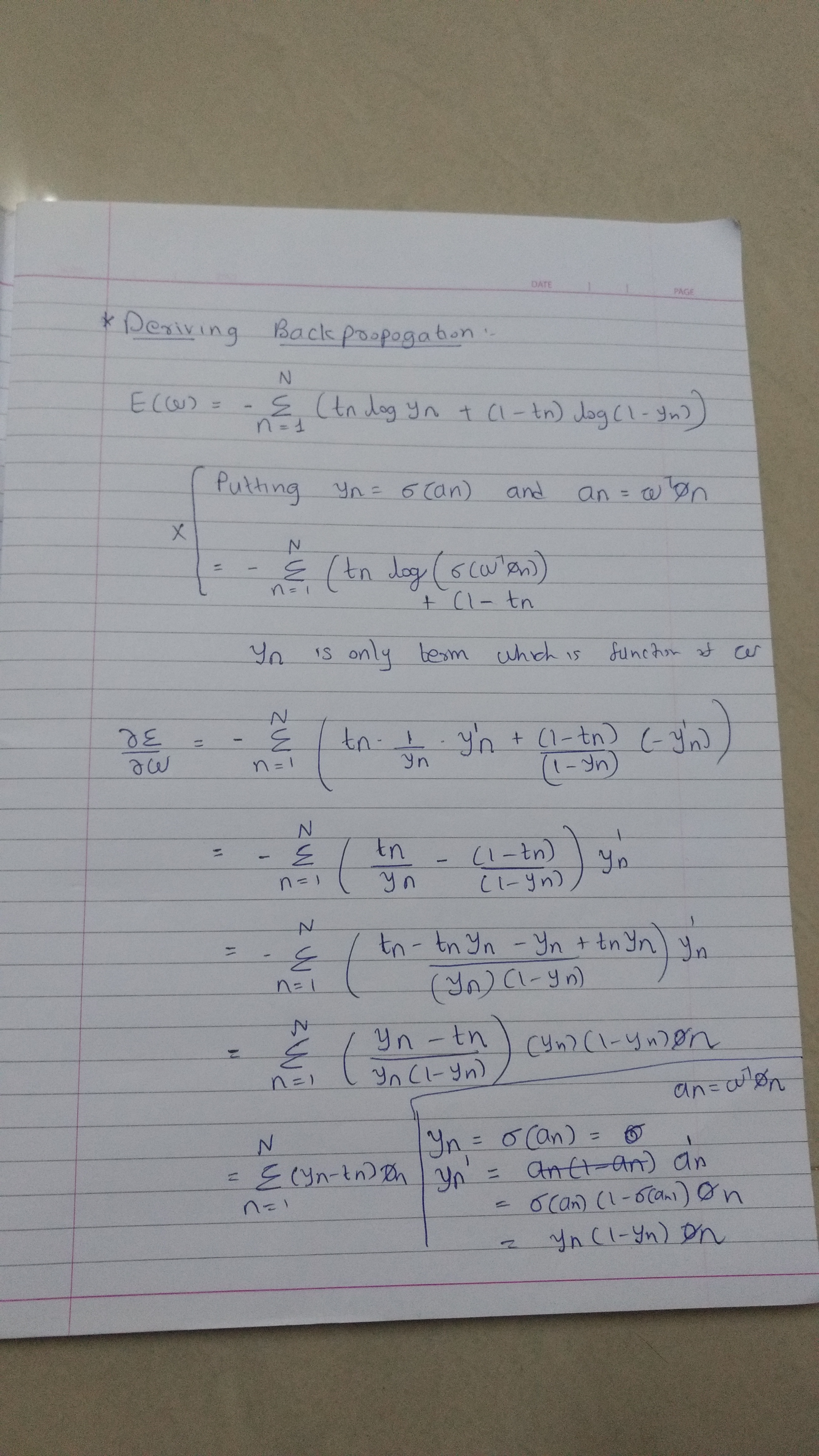
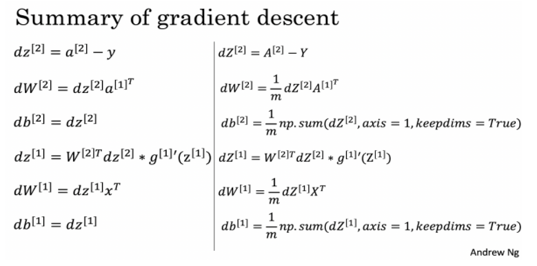
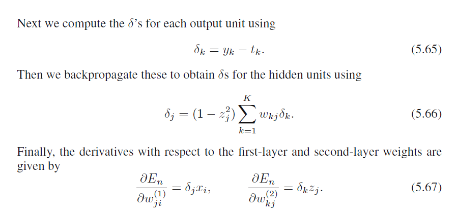
Even if you look at gradient descent below, error is multiplied by previous value. When input is higher it’s contribution to error is higher and will needs to change more.
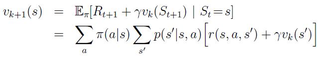
Dynamic Programming is one of the method to solve reinforcement learning problem. It assumes that complete dynamics of MDP are known and we are interested in
Finding value function for given policy (Prediction problem)
Finding optimal policy for given MDP (Control problem)
There are three things :
Policy Evaluation
We calculate value of a given state
Average value given probability all actions defined in policy
Takes Probability of actions into account
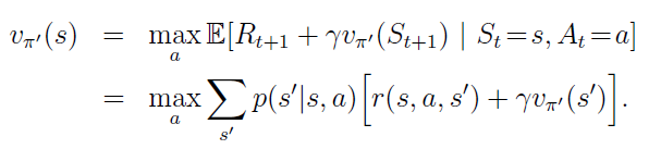
Policy Iteration
First evaluates policy
Then generates new policy based on this evaluation
Calculates and updates maximum possible value of a state
Value is maximum when we take most optimal action
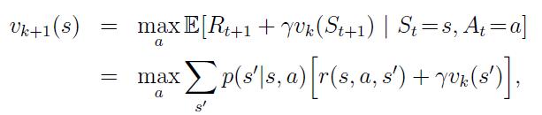
Value Iteration
Policy evaluation is time taking process
Let’s go with just one iteration
We don’t need to update policy in each iteration, just keep using new value function does the job
So it is like keep updating value function (choosing action that maximizes value instead of taking probabilities) until it converges and then selecting a policy based on this optimal values function
I have coded it at [0]
What is policy ?
A policy is simply a probability of performing an action (a) when in state (s) and our goal is to tune the policy to maximize the agents reward.
Different type of DP
Unlike traditional algo-ds problems this is a different type of dynamic programming. There mostly final ans is output of one cell, other cells are used for memoization. Here final answer is all the cells. We want to know value of all the cells. Another unusual DP problems are mentioned at [4].
Policy Evaluation
Policy Iteration
Values Iteration
Here are two slides from : http://www0.cs.ucl.ac.uk/staff/d.silver/web/Teaching_files/DP.pdf
Open AI provides framework for creating environment and training on that environment. In this post I am pasting a simple notebook for a quick look up on how to use this environments and what all functions are available on environment object.
I have used environment available on github by Denny Britz and here are the references :
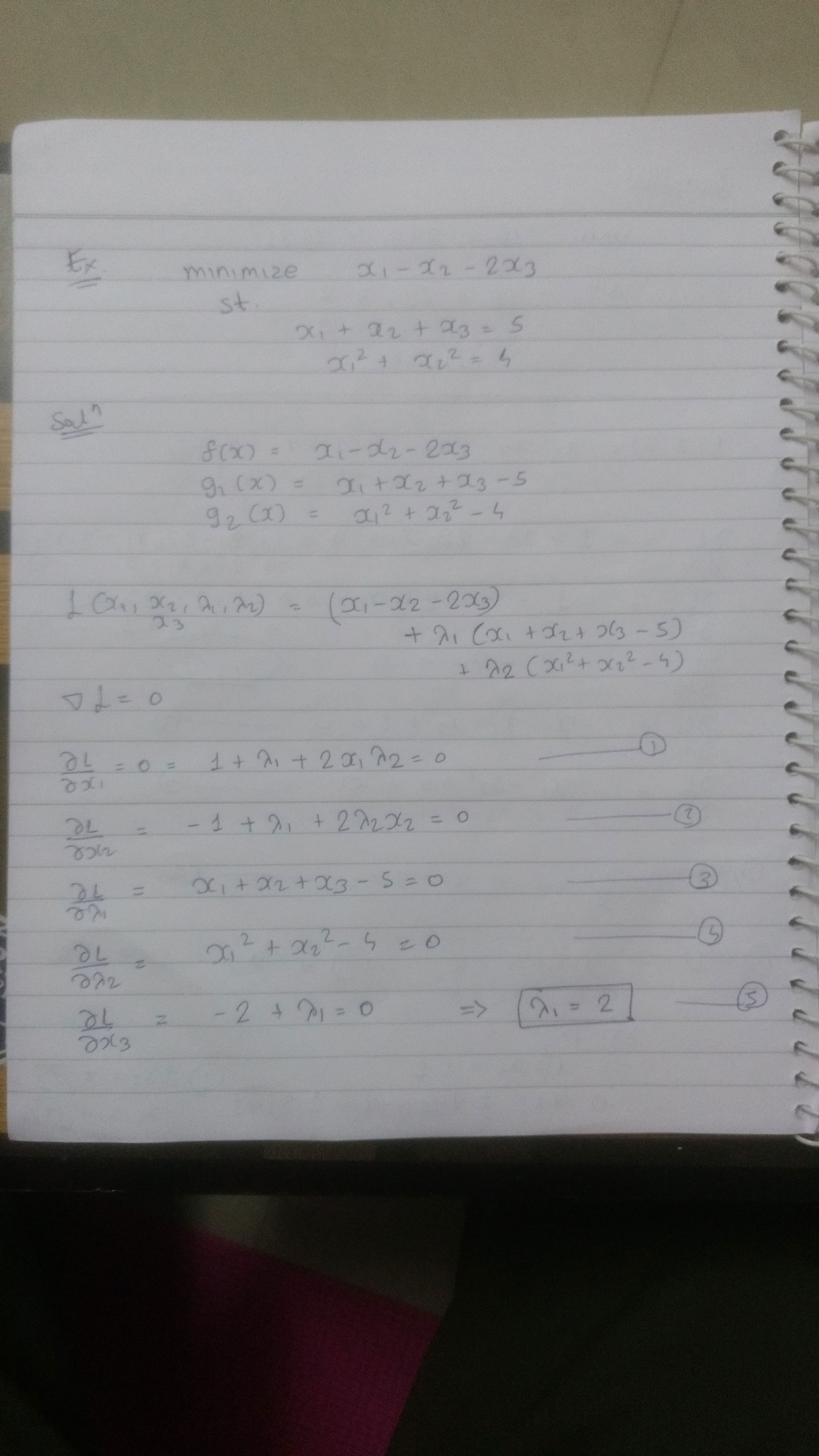
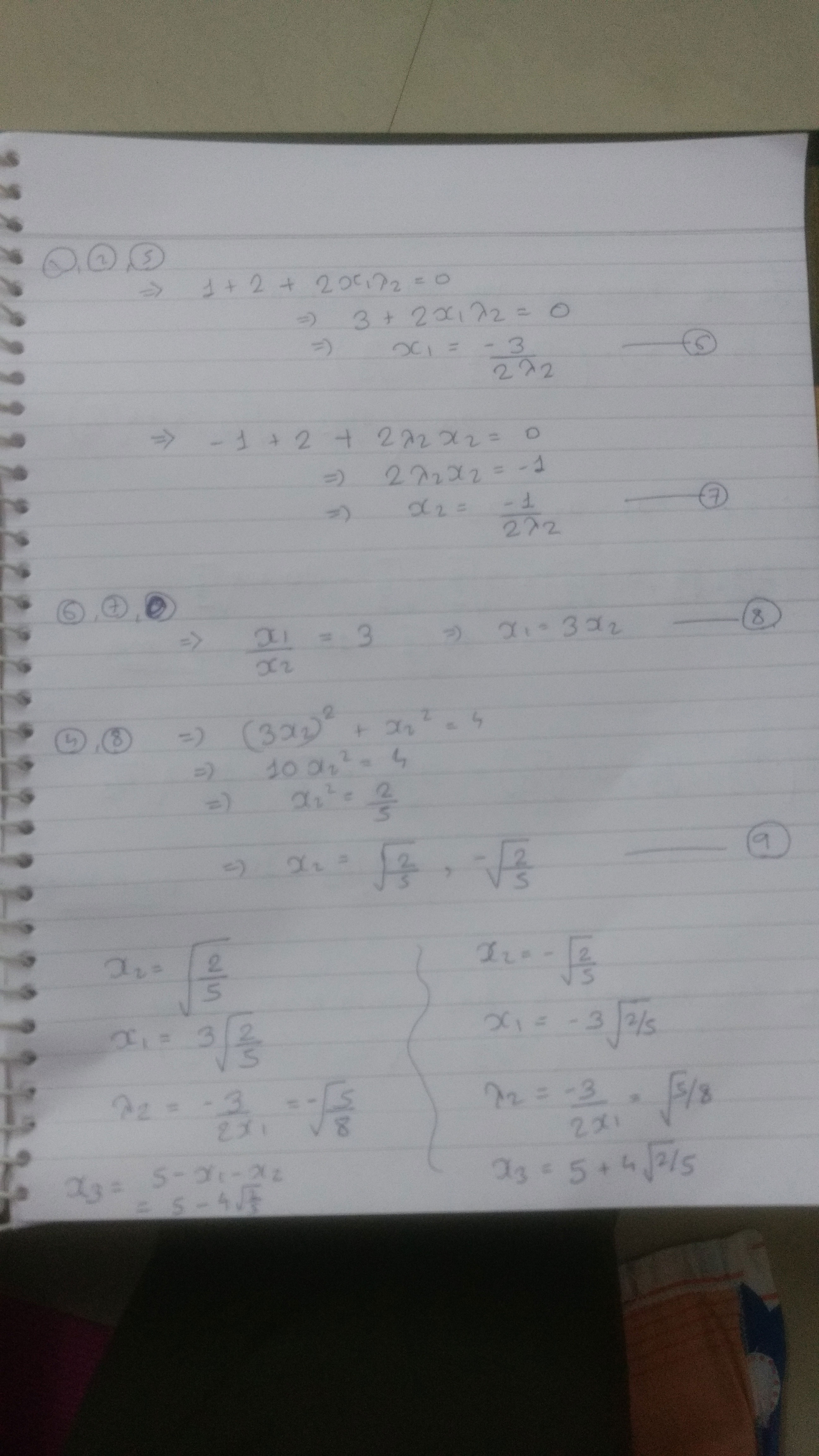
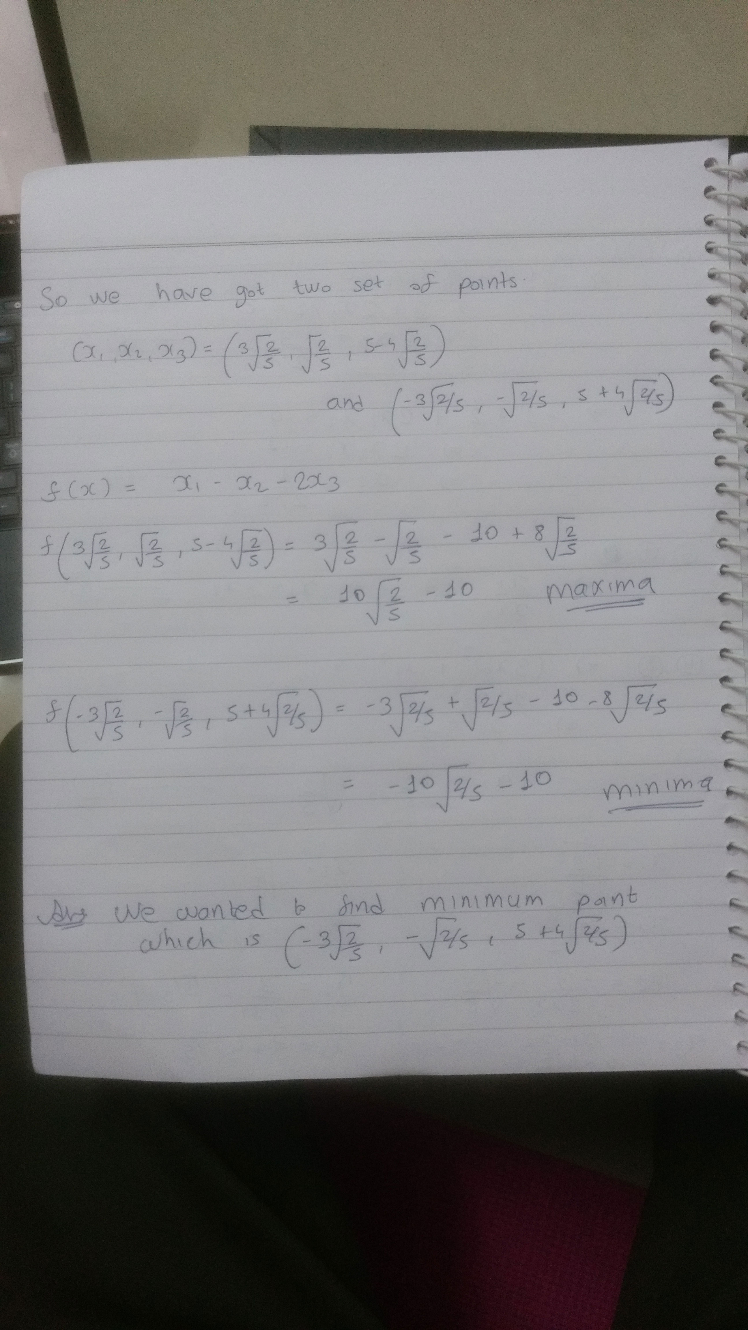
In mathematics, particularly in calculus, a stationary point or critical point of a differentiable function of one variable is a point on the graph of the function where the function’s derivative is zero. Informally, it is a point where the function “stops” increasing or decreasing (hence the name).
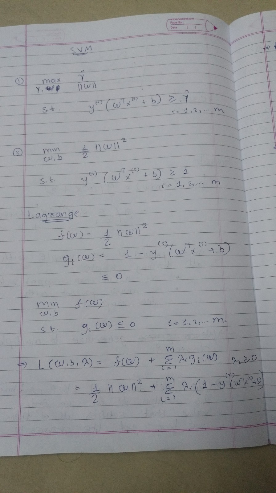
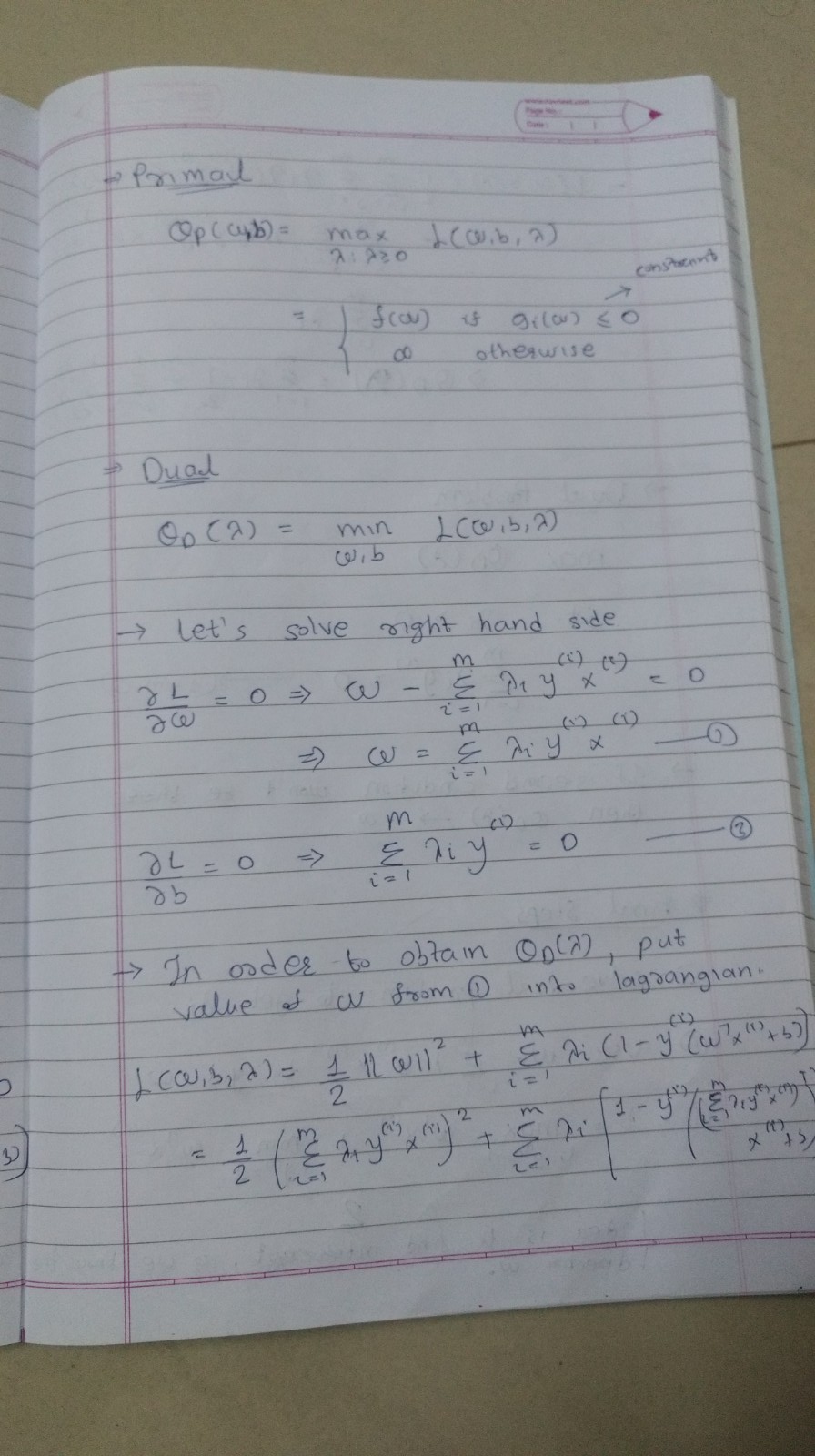
Lagrange multiplier helps us to find all the stationary points, It can be local minima, local maxima, global minima or global maxima. Once we evaluate objective function at each of these stationary point we can classify which one is local/global minima and maxima.
Thompson sampling is one approach for Multi Armed Bandits problem and about the Exploration-Exploitation dilemma faced in reinforcement learning. It is also know as posterior sampling.
Challenge in solving such a problem is that we might end up fetching the same arm again and again. Bayesian approach helps us solving this dilemma by setting prior with somewhat high variance.
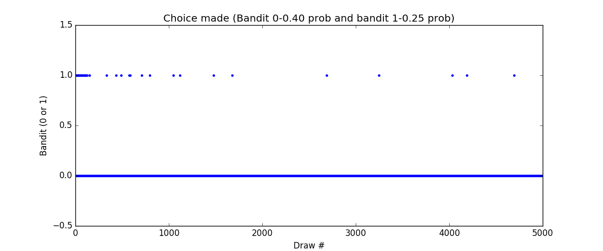
Here is the code for two armed bandit. One has success probability of 40% (bandit 0) and another has 25% (bandit 1).
We are using beta distribution for deciding which arm to pull. Beta distribution has two parameter alpha and beta. Higher values of alpha, pulls distribution towards 1. Beta distribution is always confined between 0 and 1.
How we train is that for each feedback we receive we increment alpha by 1 if it was success or beta by 1 in case of failure. For choosing the arm we draw random sample from the distribution of each arm and select the arm with highest value.
This file contains hidden or bidirectional Unicode text that may be interpreted or compiled differently than what appears below. To review, open the file in an editor that reveals hidden Unicode characters.
Learn more about bidirectional Unicode characters
And here is simulation results. We see that initially both the the armed are pulled frequently but slowly arm 1 is pulled less and less, but it is never straight away zero.
Math Behind Increasing alpha and beta
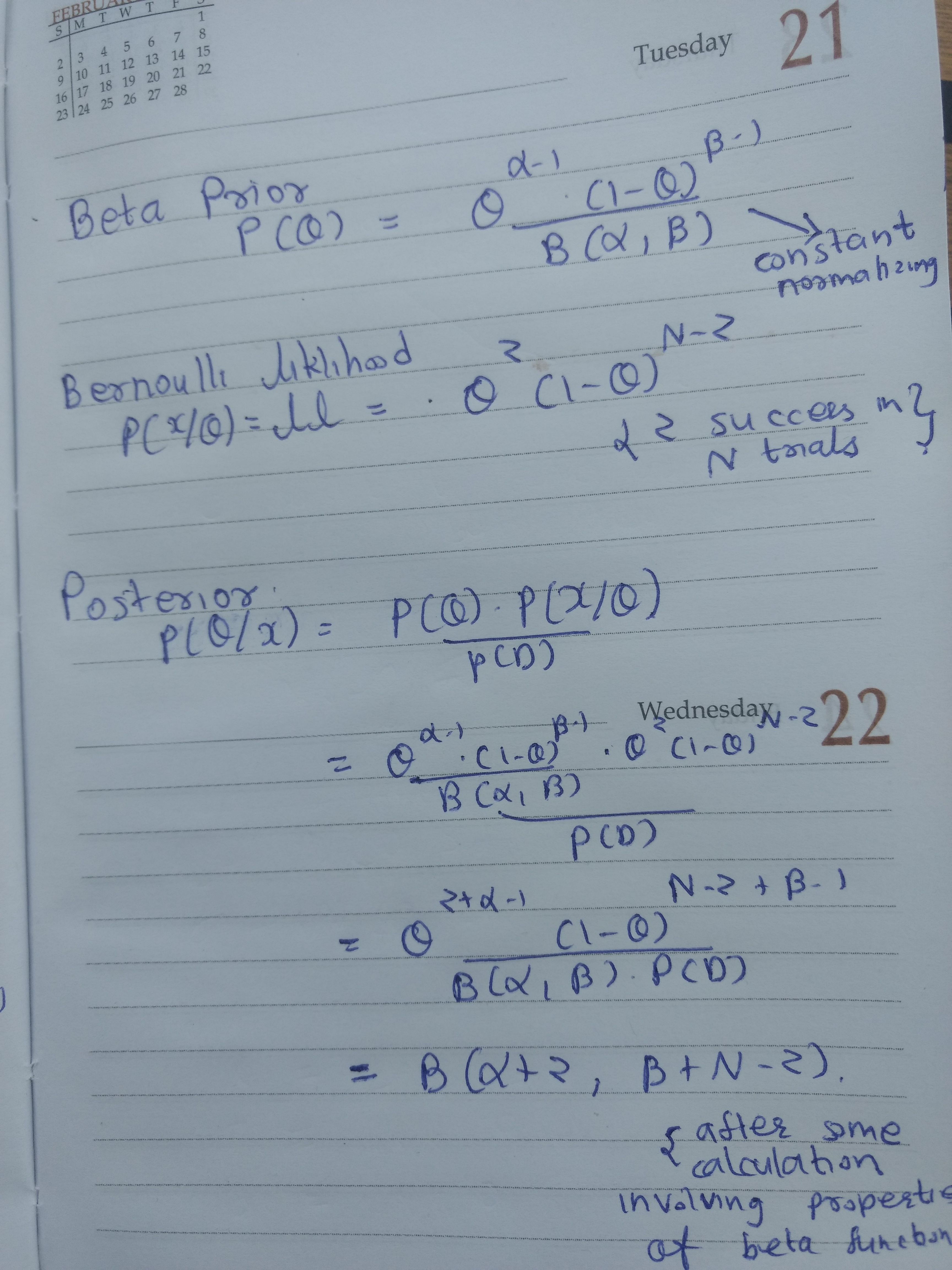
In one line posterior is beta distribution for beta prior and Bernoulli likelihood. In other words beta is a conjugate prior for Bernoulli likelihood. List of various conjugate prior is available at [1].
PDF of beta distribution is simple once you think in terms of the effect of alpha and beta.
Look at note below, formula of beta distribution is not complex, actually it is very similar to