Dynamic Programming for RL

Dynamic Programming is one of the method to solve reinforcement learning problem. It assumes that complete dynamics of MDP are known and we are interested in

  • Finding value function for given policy (Prediction problem)
  • Finding optimal policy for given MDP (Control problem)


There are three things :

  • Policy Evaluation
    • We calculate value of a given state
      • Average value given probability all actions defined in policy
    • Takes Probability of actions into account
  • Policy Iteration
    • First evaluates policy
    • Then generates new policy based on this evaluation
    • Calculates and updates maximum possible value of a state
      • Value is maximum when we take most optimal action
  • Value Iteration
    • Policy evaluation is time taking process
    • Let’s go with just one iteration
    • We don’t need to update policy in each iteration, just keep using new value function does the job
    • So it is like keep updating value function (choosing action that maximizes value instead of taking probabilities) until it converges and then selecting a policy based on this optimal values function
    • I have coded it at [0]


What is policy ?

A policy is simply a probability of performing an action (a) when in state (s) and our goal is to tune the policy to maximize the agents reward.


Different type of DP

Unlike traditional algo-ds problems this is a different type of dynamic programming. There mostly final ans is output of one cell, other cells are used for memoization. Here final answer is all the cells. We want to know value of all the cells. Another unusual DP problems are mentioned at [4].


Policy Evaluation

policy_eval

Policy Iteration

policy_iter

Values Iteration

value_iter


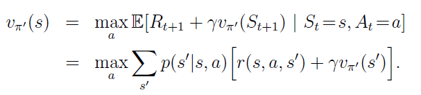
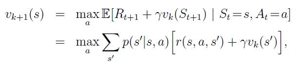
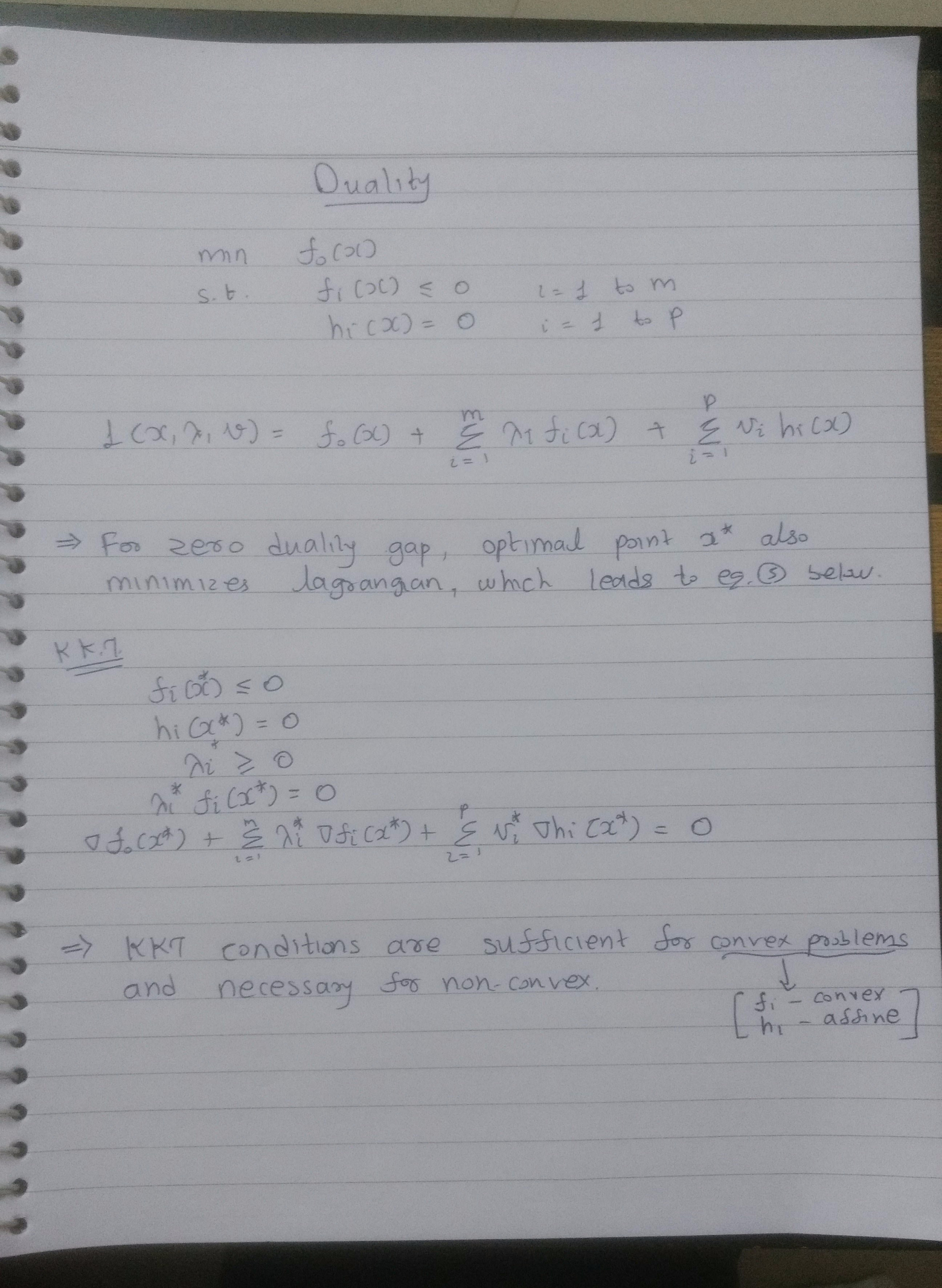
Here are two slides from : http://www0.cs.ucl.ac.uk/staff/d.silver/web/Teaching_files/DP.pdf


References

[0] : https://github.com/arcarchit/datastories/blob/master/RL_GridWorld.ipynb

[1] : Sutton’s book

[2] : https://github.com/dennybritz/reinforcement-learning/tree/master/DP/

[3] : http://www0.cs.ucl.ac.uk/staff/d.silver/web/Teaching_files/DP.pdf

[4] : https://github.com/arcarchit/mit-ds-algo/blob/master/dsalgo/cs/dp/dp_equations.md
OpenAI Gym Environment

Open AI provides framework for creating environment and training on that environment. In this post I am pasting a simple notebook for a quick look up on how to use this environments and what all functions are available on environment object.

I have used environment available on github by Denny Britz and here are the references :

References :

https://github.com/dennybritz/reinforcement-learning

Learning Reinforcement Learning (with Code, Exercises and Solutions)

https://gym.openai.com/docs/

My Code : https://gist.github.com/arcarchit/2b3363e2615df7ef5c8d4941d4dfa9e8


Loading

Sorry, something went wrong. Reload?
Sorry, we cannot display this file.
Sorry, this file is invalid so it cannot be displayed.

view raw

gym_env.ipynb

hosted with ❤ by GitHub

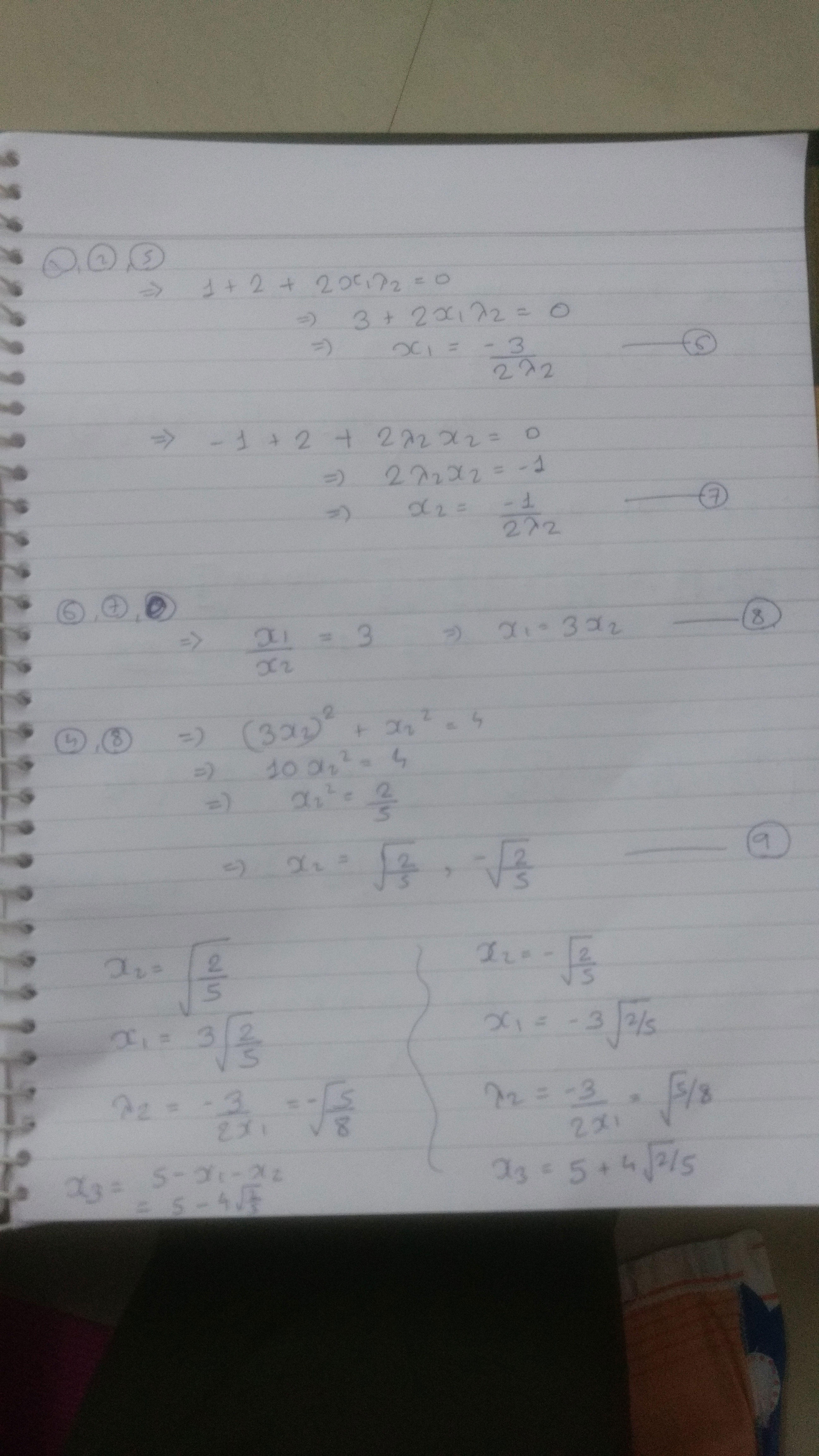
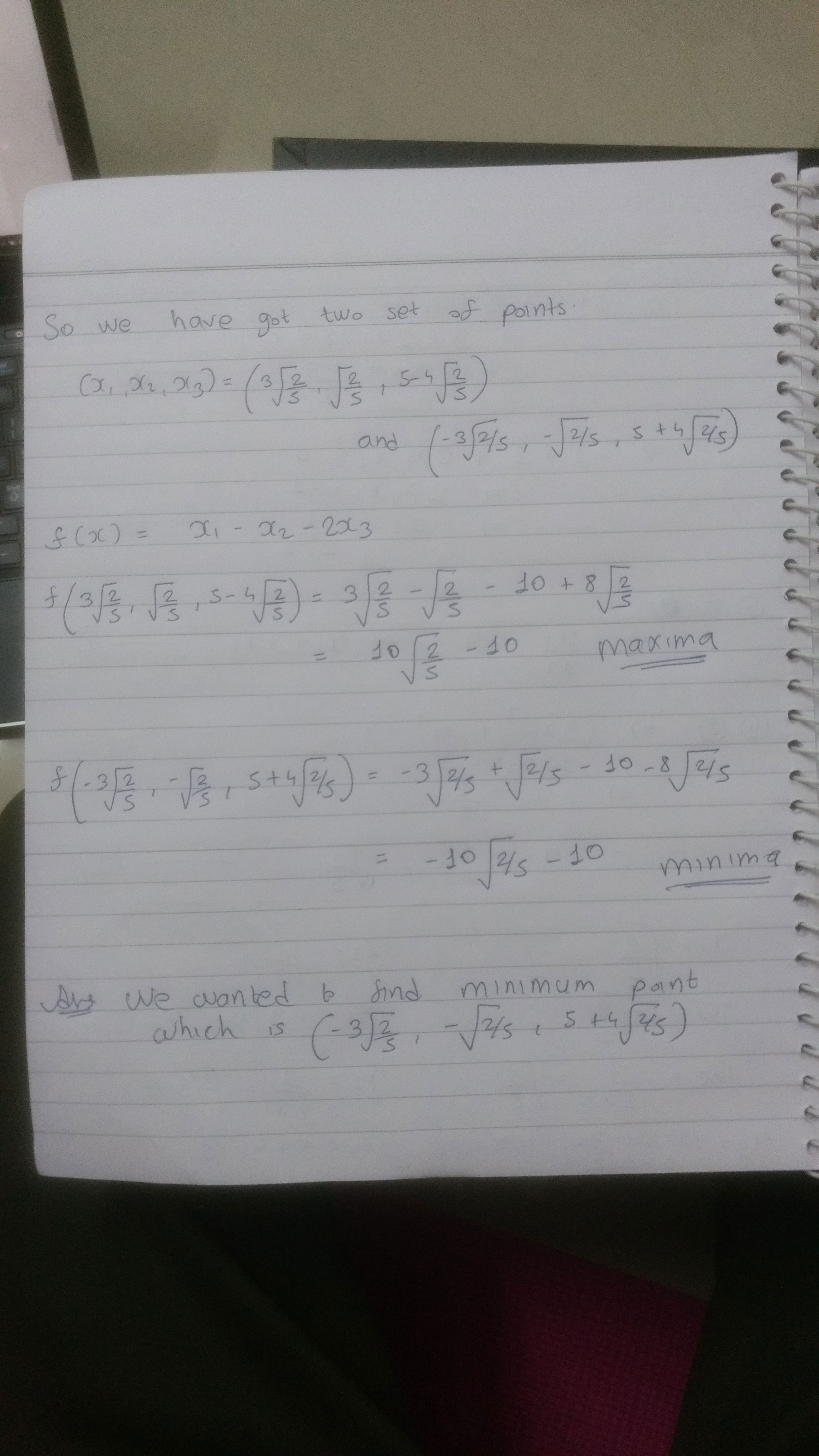
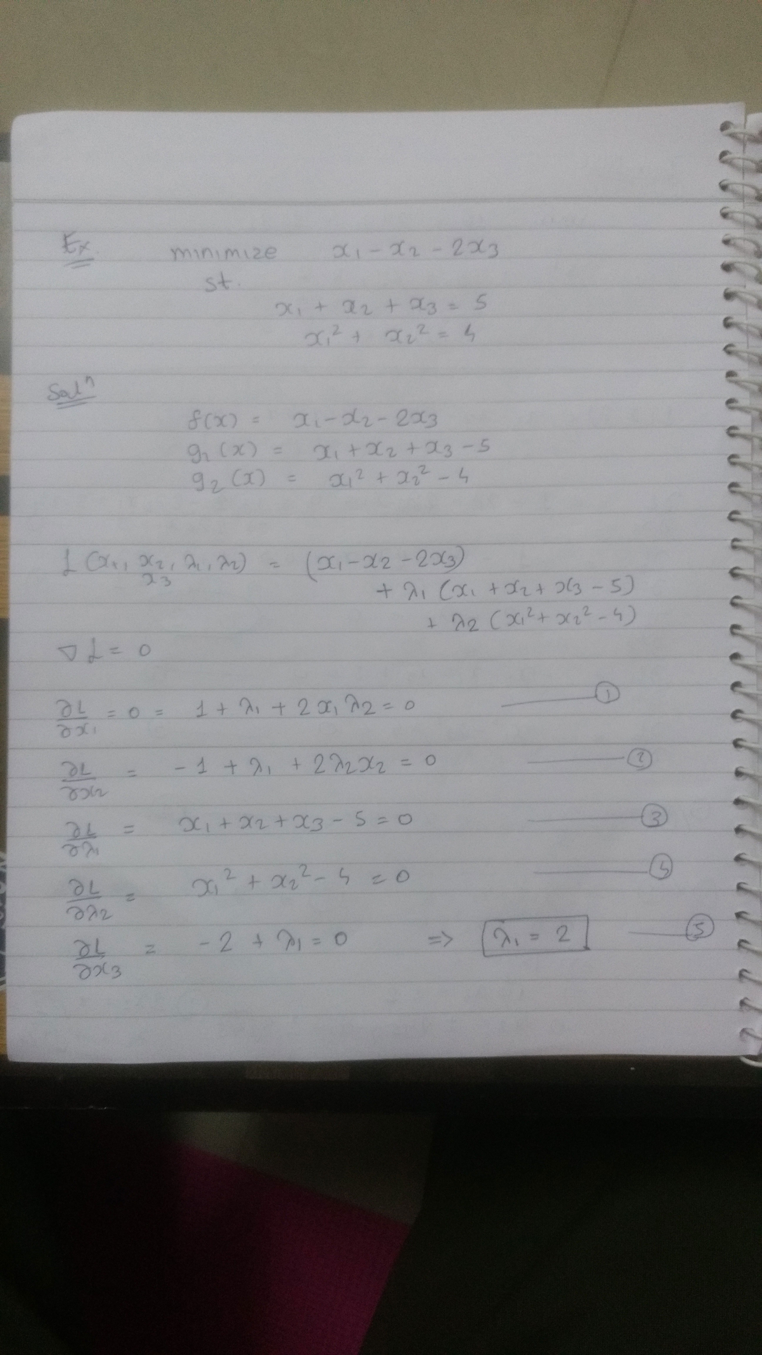
[Example] Lagrange Multiplier With Equality Constraints


Stationary Point

Definition of stationary point from wikipedia :

In mathematics, particularly in calculus, a stationary point or critical point of a differentiable function of one variable is a point on the graph of the function where the function’s derivative is zero. Informally, it is a point where the function “stops” increasing or decreasing (hence the name).


Lagrange multiplier helps us to find all the stationary points, It can be local minima, local maxima, global minima or global maxima. Once we evaluate objective function at each of these stationary point we can classify which one is local/global minima and maxima.


Example


Thompson Sampling

Thompson sampling is one approach for Multi Armed Bandits problem and about the Exploration-Exploitation dilemma faced in reinforcement learning. It is also know as posterior sampling.

Challenge in solving such a problem is that we might end up fetching the same arm again and again. Bayesian approach helps us solving this dilemma by setting prior with somewhat high variance.

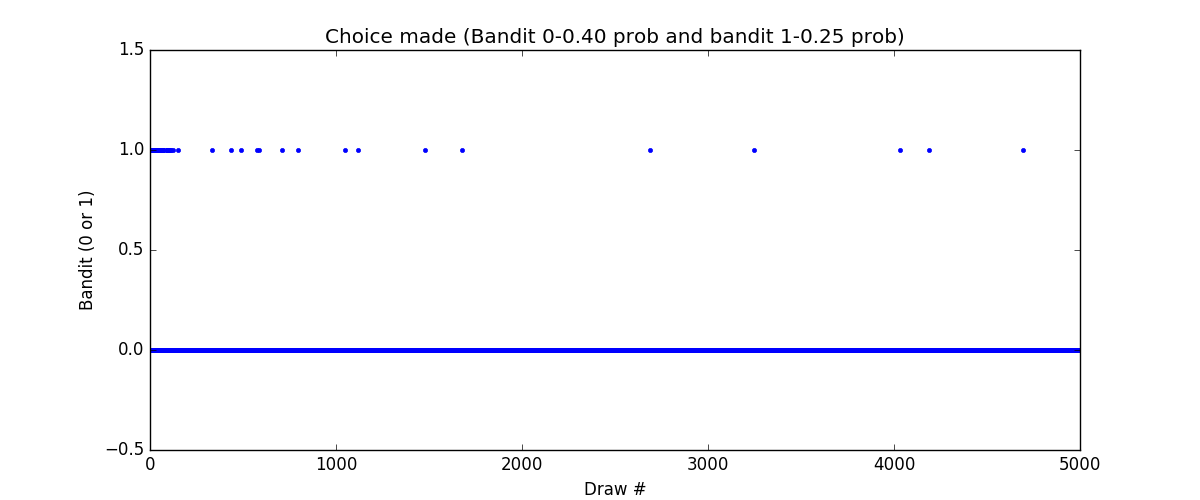
Here is the code for two armed bandit. One has success probability of 40% (bandit 0) and another has 25% (bandit 1).

We are using beta distribution for deciding which arm to pull. Beta distribution has two parameter alpha and beta. Higher values of alpha, pulls distribution towards 1. Beta distribution is always confined between 0 and 1.

How we train is that for each feedback we receive we increment alpha by 1 if it was success or beta by 1 in case of failure. For choosing the arm we draw random sample from the distribution of each arm and select the arm with highest value.

import numpy as np
import scipy.stats as stats
from matplotlib import pyplot as plt
class BetaThompson:
def __init__(self, num_bandits, prior_a, prior_b):
self.num_bandits = num_bandits
self.a = prior_a
self.b = prior_b
def learn(self, bandit, success):
if success:
self.a[bandit]+=1
else:
self.b[bandit]+=1
def suggest(self):
sampled_prob = []
for i in range(self.num_bandits):
dist = stats.beta(self.a[i], self.b[i])
prob=dist.rvs()
sampled_prob+=[prob]
return sampled_prob.index(max(sampled_prob))
class Gamble:
def __init__(self, num_bandits, binom_mean):
self.num_bandits=num_bandits
self.binom_mean=binom_mean
def gamble(self, bandit_no):
dist=stats.binom(n=1,p=self.binom_mean[bandit_no])
success = True if dist.rvs()>0.5 else False
return success
def main():
g = Gamble(2, [0.40, 0.25])
bot = BetaThompson(2, [1,1], [1,1])
choice=[]
for i in range(5000):
suggestion = bot.suggest()
result = g.gamble(suggestion)
bot.learn(suggestion, result)
choice+=[suggestion]
plt.figure(figsize=(12,5))
plt.plot(choice, 'b.')
plt.ylim([-0.5,1.5])
plt.title('Choice made (Bandit 0-0.40 prob and bandit 1-0.25 prob)')
plt.xlabel('Draw #')
plt.ylabel('Bandit (0 or 1)')
plt.savefig('choice.png')
if __name__== "__main__":
main()

And here is simulation results. We see that initially both the the armed are pulled frequently but slowly arm 1 is pulled less and less, but it is never straight away zero.

choice

Math Behind Increasing alpha and beta

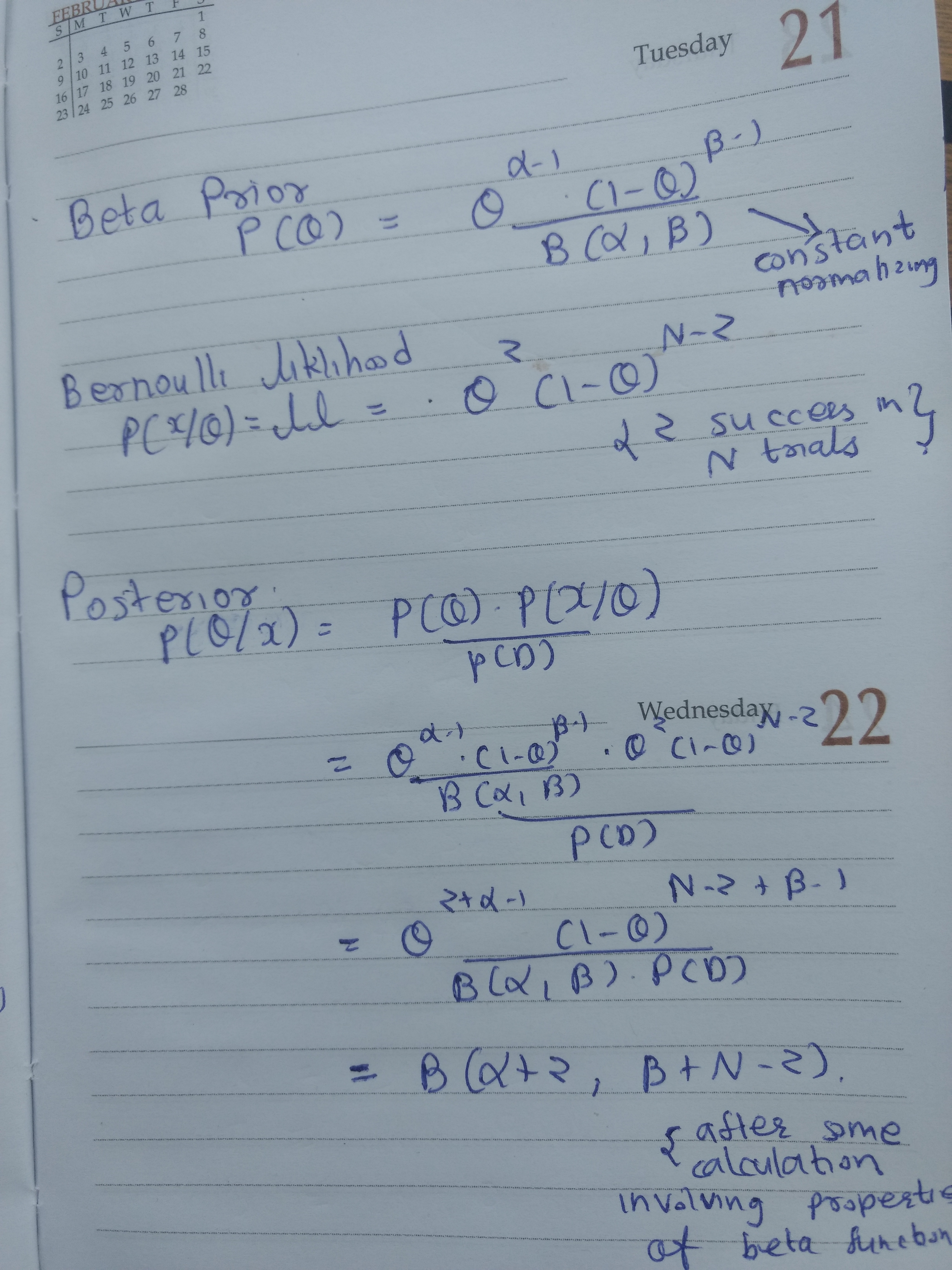
In one line posterior is beta distribution for beta prior and Bernoulli likelihood. In other words beta is a conjugate prior for Bernoulli likelihood. List of various conjugate prior is available at [1].

PDF of beta distribution is simple once you think in terms of the effect of alpha and beta.

Look at note below, formula of beta distribution is not complex, actually it is very similar to

bayesian

References

[1] : https://ocw.mit.edu/courses/mathematics/18-05-introduction-to-probability-and-statistics-spring-2014/readings/MIT18_05S14_Reading15a.pdf

Deep learning taking off

I recently started Andrew Ng’s specialization on deep learning and found these two interesting points :

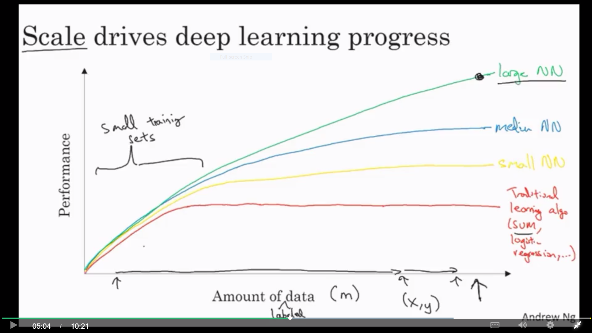
One is about how performance of algorithm changes with the amount of data. Traditional algorithms have limits but Deep neural network has more advantages.

whyD


Also for the small amount of data traditional algorithms may win over neural nets with good feature engineering.

Second reason is that deep learning requires data, computation and efficient algorithms. Recent years have seen significant advancement in algorithm to increase computation efficiency. For example sigmoid to ReLU was an algorithmic change which allowed gradient to converge faster.


Ref : https://www.coursera.org/learn/neural-networks-deep-learning/home

Lagrange Duality

There are three things :

  1. Original problem (Primal problem)
  2. Dual function (Function of lagrange multiplier)
  3. Dual problem


Suppose p is the solution of primal problem and d the dual problem.


If original problem is minimization, we are interested in lower bound (d) such that d<p.  We want to find maximum value of d and dual problem becomes maximization problem.


If original problem is maximization, we are interested in finding upper bound (d) such that p<d. We want to find minimum value of d and dual problem become minimization problem.


Dual problem is always convex irrespective of primal problem.


d<p is weak duality, while d=p is strong duality.

If primal problem is convex strong duality generally holds.

Slater’s condition is sufficient tests for convex optimization.


Further reading :

Kanpsack Problem here 

Convex Optimization by Stephen Boyd


Parametric and Nonparametric tests

We rarely heard of nonparametric tests while reading standard statistical books. However there are some scenarios where they should be used instead of parametric tests. [1] has beautiful blog about it, I am putting just a summary from that.


Different Tests

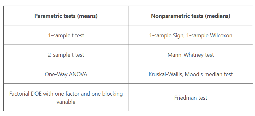
Table below displays various tests, I have verified that all of these tests are available in python stats package.

tests_1

When to Use Parametric Tests

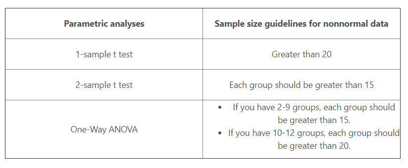
  • Parametric tests can perform well with skewed and nonnormal distributions
    • It is important to follow guidance in the sample size of data as shown in table below
  • Parametric tests can perform well when the spread/variance of each group is different
  • It has Statistical power

tests_2

Reasons to Use Nonparametric Tests

  • Your area of study is better represented by the median
    • Income distribution is skewed and median is more useful than mean
    • Few billionaires can boost up the mean significantly
  • You have a very small sample size
    • Even less than what is mentioned in table above
  • You have ordinal data, ranked data, or outliers that you can’t remove


References:

[1] : http://blog.minitab.com/blog/adventures-in-statistics-2/choosing-between-a-nonparametric-test-and-a-parametric-test

[Theory] Lagrange Multiplier and Constrained Optimization

Lagrange multipliers helps us to solve constrained optimization problem.

An example would to maximize f(x, y) with the constraint of g(x, y) = 0.

Geometrical intuition is that points on g where f either maximizes or minimizes will have a parallel gradient of f and g

∇ f(x, y)  =  λ ∇  g(x, y)

We need three equations to solve for x, y and λ.

Solving above gradient with respect to x and y gives two equation and third is g(x, y) = 0

These will give us the point where f is either maximum or minimum and then we can calculate f manually to find out point of interest.

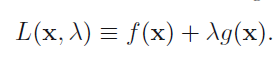
Lagrange is a function to wrap above in single equation.

L(x, y, λ) = f(x, y) – λ g(x, y)

And then we solve ∇ L(x, y, λ) = 0


Budget Intuition

Let f represent the revenue R and g represent cost C.

Also let g(x, y) = b where b is maximum cost that we can afford.

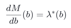
Let M* be the optimized value obtained by solving lagrangian and value of λ we got was λ*.

l1

So λ is the rate with which maximum revenue will increase with unit change in b.


Inequality Constraint


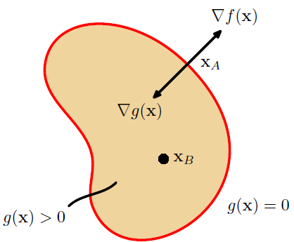
Here is the problem of finding maximum of f(x) [2]

l5

l4
l7

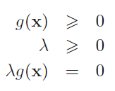
Above conditions are known as Karush-Kuhn-Tucker (KKT) conditions.

First – primal feasibility

Second – dual feasibility

Third  –  complementary slackness conditions

For the problem of finding minimum value of f(x) we minimize following with same KKT conditions:

l9


This can be extended to arbitrary number of constraints.

l8


Notes

  • This is relates to solving the dual of a problem for convex function as we had in Boyd’s book
  • For unconstrained optimization computing hessian of a matrix is one way of solving if it is continuous  [1]


formal summary

References

[0] https://www.khanacademy.org/math/multivariable-calculus/applications-of-multivariable-derivatives/constrained-optimization/a/lagrange-multipliers-single-constraint

[1] https://www.youtube.com/watch?v=TyfZaZSF5nA

[2] Pattern Recognition and machine learning by Bishop

On multivariate Gaussian

Formulas

Formula for multivariate gaussian distribution

g1

Formula of univariate gaussian distribution

g2

Notes:

  • There is normality constant in both equations
  • Σ being a positive definite ensure quadratic bowl is downwards
  • σ2 also being positive ensure that parabola is downwards

On Covariance Matrix

Definition of covariance between two vectors:

g3

When we have more than two variable we present them in matrix form. So covariance matrix will look like

g4

  • Above is very similar to how we compute sigma^2 in 1-D = (x – mu)^2
  • Formula of multivariate gaussian distribution demands Σ to be singular and symmetric positive semidefinite, which in terms means sigma will be symmetric positive semidefinite.
  • For some data above demands might not meet

Side Note

  • Covariance is directional measure
  • Correlation is scaled measure
    • We normalise by individual variance

Derivations

Following derivations  are available at [0]:

  • We can prove[0] that when covariance matrix is diagonal (i.e there is variables are independent) multivariate gaussian distribution is simply multiplication of single gaussian distribution of each variable.
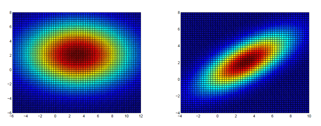
  • It was derived that shape of isocontours (figure 1) is elliptical and axis length is proportional to individual variance of that variable
  • Above is true even when covariance matrix is not diagonal and for dimension n>2 (ellipsoids)

g5

Notes and example of bi-variant Gaussian

https://github.com/arcarchit/datastories/blob/master/notes/bivariant_gaussian.pdf

First part above says that bi-variant destitution can be generated from two standard normal distribution z = N(0,1).

For any given k-variant Gaussian we can represent it as linear combination of k standard normal distribution. One simpler way to find these coefficient is Cholesky decomposition. Theorem 1 below stats the same thing.

This has a reference from [1].

Linear Transformation Interpretation

g6

This was proved in two steps [0]:

Step-1 : Factorizing covariance matrix

g7

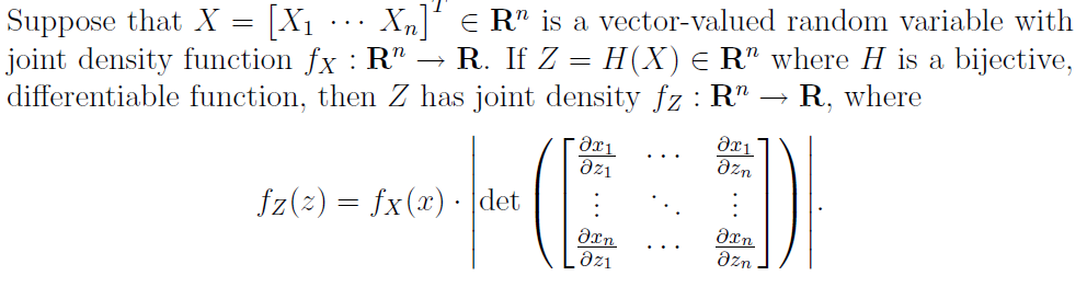
Step-2 : Change of variables, which we apply to density function

g8

On Practical Example

Height, wight and waist size of men in US (Of course it weight can be negative, so it is approximately normal)

References

[0] http://cs229.stanford.edu/section/gaussians.pdf

[1] https://www2.stat.duke.edu/courses/Spring12/sta104.1/Lectures/Lec22.pdf