Classification – One vs Rest and One vs One

June 11, 2017May 21, 2023Archit Vora 1 Comment

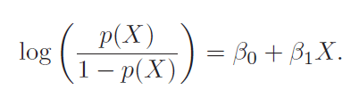
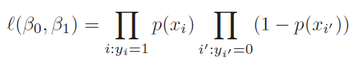
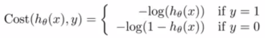
In the blog post on Cost Function And Hypothesis for LR we noted that LR (Logistic Regression) inherently models binary classification. Here we will describe two approaches used to extend it for multiclass classification.

One vs Rest approach takes one class as positive and rest all as negative and trains the classifier. So for the data having n-classes it trains n classifiers. Now in the scoring phase all the n-classifier predicts probability of particular class and class with highest probability is selected.

One vs One considers each binary pair of classes and trains classifier on subset of data containing those classes. So it trains total n*(n-1)/2 classes. During the classification phases each classifier predicts one class. (This is contrast to one vs rest where each classifier predicts probability). And the class which has been predicted most is the answer.

Example

For example consider four class problem having classes A, B, C, and D.

One vs Rest

Models classifiers_A, classifier_B, classifier_C and classifier_D
During prediction here is the probability we get:
- classifier_A = 40% = prob(class A)
- classifier_B = 30%
- classifier_C = 60%
- classifier_D = 50%
We assign it class B
Note that Summation might not be come out to 1
- Prob(class A) + Prob(class B) + Prob(class C)

One vs One

We train total six classifier with subset of data containing classes involved
- classifier_AB
- classifier_AC
- classifier_AD
- classifier_BC
- classifier_BD
- classifier_CD
And during classification
- classifier_AB assigns class A
- classifier_AC assigns class A
- classifier_AD assigns class A
- classifier_BC assigns class B
- classifier_BD assigns class D
- classifier_CD assigns class C
We assign it to class A
How do we estimate Prob(class A) ?
- Somewhat complicated

More notes

One vs rest trains less no of classifier and hence is faster overall and hence is usually prefered
Single classifier in one vs one uses subset of data, so single classifier is faster for one vs one
One vs one is less prone to imbalance in dataset (dominance of particular classes)

Inconsistency

What if two class gets equal vote in the case of one vs one case
What if probability are almost close to equal in case of one vs rest
We will discuss this issue in further blog posts

On Classification Accuracy

June 10, 2017October 25, 2020Archit Vora 3 Comments

Edit : Extended post is available here

Some Scenarios

In finance default is failure to meet the legal obligation of loan. Given some data we want to classify whether the person will be defaulter or not.
- Suppose our training data-set is imbalanced. Out of 10k samples only 300 are defaulters. (3%)
- Classifier in the following table is good at classifying non defaulters but not good at classifying defaulters (which is more important for credit card company)
- Assume what if out of 300 defaulters 250 are classified as non defaulters and given the credit card
Doctors want to conduct a test whether a patient has cancer or not.
- Popular terms in medical field are sensitivity and specificity
- Instead of trying to classify person as defaulter, here we classify if patient has cancer.
- Sensitivity = 81/333 = 24 %
- Specificity = 9644/9667 = 99 %
- Every medical test thrives to achieve 100% in both sensitivity and specificity.
In information retriever we want to know how many % of relevant pages we were able to retrieve.
- TP = 81
- FP = 23
- TN = 9644
- FN = 252
- Precision = 81/104= 77%
- Recall = 81/333= sensitivity = 24%

Example

Formulas:
- Precision = TP/(TP+FP)
- Recall = TP/(TP+FN)
- Sensitivity = TP/(TP+FN)
- Specificity = TN/(TN+FP)
- Recall and sensitivity are same

Solution is to change the threshold

Earlier we were assigning person to default if probability is more than 50%
Now we want to assign more person as defaulter
So we will assign them to defaulter when probability is more than 20%
This will incorrectly classify non-defaulters to defaulters but that is less concerned compared to assigning defaulter to non-defaulter
- This will also increase the overall error rate, which is still okay

ROC and AUC

We can always increase sensitivity by classifying all samples as positive
We can increase specificity by classifying all samples as negative
ROC plot (sensitivity) vs (1-specificity)
- That is TP vs FP
- And also precision vs recall
ROC = Receiver operating characteristic
It is good to have ROC curve on top left
- Better classifier
- Accurate test
And ROC curve close to 45 degree represents less accurate test
AUC = Area Under Curve
- Area under ROC curve
Ideal value for AUC is 1
AUC of 0.5 (45 degree line) represents a random classifier

How to plot ROC?

Change the probability threshold from 0 to 1 and measure sensitivity and specificity. If specificity keeps on decreasing ((100-specificity) keeps on increasing) as sensitivity increase it is a bad classifier.
For random classifier ROC is 45 degree line
- You draw random number between (0, 1)
- Classify it based on threshold
- So threshold is there
- But while building classifier we want to do better than drawing random probability between (0, 1). We also want to consider features into account while drawing between (0, 1)
Can AUC be less than 0.5? I don’t think so.
- Complementing the output will bring it to other side of line anyway.
What if I classified all of them as positive?
- That means you are taking all 1. You can not plot ROC with that.

Threshold selection

Unless there is special business requirement (as in credit card defaulters) we want to select a threshold which maximizes TP while minimizing FP
There are two methods to do that:
- Point which is closest to (0, 1) in ROC curve
- Youden Index
  - Point which maximizes vertical distance from line of equality (45 degree line)
  - We can derive that this is the point which maximizes (sensitivity + specificity)

AUC vs overall accuracy as comparison metric

AUC helps us understand how much our classifier is away from random guess, which accuracy can not tell
Accuracy is measured at particular threshold while AUC requires moving threshold from 0 to 1

F score

We know that recall and sensitivity are same, but precision and specificity are not same
While medical field is more concerned about specificity, information retrieval is more concerned about precision
So they came up with F score which is harmonic mean of precision and recall
AUC helps us maximizing sensitivity and specificity simultaneously while F score helps us maximizing precision and recall simultaneously
Beta in f score helps providing weight to precision and recall.
Harmonic mean can not be made arbitrarily large while changing some values to bigger one and leaving at least one unchanged. It is maximizes when all elements are increased.
- x = 0, y = 1 will give 0.5 in arithmetic mean but is zero for harmonic mean

harmonic mean

References

Assessing and Comparing Classifier Performance with ROC Curves

Click to access roccurve.pdf

https://www.medcalc.org/manual/roc-curves.php

https://en.wikipedia.org/wiki/F1_score

An Introduction to Statistical Learning – http://www-bcf.usc.edu/~gareth/ISL/

https://stats.stackexchange.com/questions/221997/why-f-beta-score-define-beta-like-that

https://en.wikipedia.org/wiki/Harmonic_mean

Cost Function And Hypothesis for Logistic Regression

June 8, 2017May 17, 2023Archit Vora 3 Comments

Hypothesis

We want a hypothesis that is bounded between zero and one, regression hypothesis line extends beyond this limits. Hypothesis here also represents probability of observing an outcome.

Hypothesis by ISLR and Andrew N.G :

Odds and log-odds/logit

Log of odd is also called logit. So above is logit(p(x)) = b0 + b1X.

In terms of GLM we call it a logic link function. Logit has a property of broadcasting [0,1] range to [-inf, inf]. Log does not have that property.

In regression beta1 given average change in y for unit change in x. But here it says unit increase in x changes log-odds by beta1. It multiplies odds by exp(beta1) and hence depends on current value of odds and therefor is not linear.

Cost Function

For ISLR perspective it is likelihood that we want to maximize.

Andre N.G looks it from the perspective of modifying cost function of linear regression.

As we can see that Andrew N.G cost function is same as maximizing log likelihood of ISLR.

Least square in case of linear regression is special case of maximum likelihood. We know that derivation where we assume likelihood to be gaussian.

Logistic Regression For well separated classes

MLE estimation becomes unstable when classes are well separated. While this is acceptable for classification tasks, it is not ideal for risk estimation. Regularization techniques can help avoid this instability. Support Vector Machines (SVM) also perform well for well-separated classes. As shown in figure below[1], the intercept of the sigmoid function reaches -inf, and the slope reaches inf. This allows the slope to come from an infinitely weighted feature.

Why Can’t we use square loss ?

Labels (+1, and -1)
Prediction : +1 when w*x > 0 else -1
Consider scenario [2]
- label +1
- w*x = 100
- Prediction is correct
- Still we add it to loss (100-1)^2
Solutions are hinge loss and logistic loss

Why is not logistic loss not 0 for correct prediction ?
- There are more training samples. We want to find parameter such that it balances all of them
- If we make it 0 positive examples would no longer contribute to loss (like SVM)
  - That’s why hinge loss create support vectors. More about that on SVM’s blog post
- Also this is the property which will make coefficient higher for well separated classes
  - To control that we use regularisation
  - Regularisation is while training, not while prediction, we are just changing loss function
  - Predict is still +1 is w*x > 0 else -1

Why can’t we use step loss ?

When we are incurring loss, we also want to know which direction to go to reduce loss.
Gradient/slope is what provide this information. [2]
Step loss (0-1) has zero gradient

Reference

[1] https://stats.stackexchange.com/questions/254124/why-does-logistic-regression-become-unstable-when-classes-are-well-separated

[2] Notes of different loss function is taken from Mike Galbart’s course – https://github.com/UBC-CS/cpsc340/blob/master/lectures/L19demo.ipynb

Hypothesis and T-Distribution

March 14, 2017May 17, 2023Archit Vora Leave a comment

We calculate the t-score using hypothesis data, which also provides us with the degrees of freedom. This value is then supplied to a function that gives us the probability of the hypothesis being true.

The t-test can be seen as a ratio, similar to a signal-to-noise ratio. The numerator allows us to center it around zero, while the denominator represents the standard error of the mean (SEM) calculated as s/sqrt(n), where s is the standard deviation of the samples.

The t-score indicates how many SEM the current mean is away from the mean given in the hypothesis. If it is far away, it suggests a low probability of the null-hypothesis-mean being true, leading us to reject the null hypothesis.

In engineering, we typically assume that the mean and standard deviation are given and true, and we compute the probability of observing the sample. However, in hypothesis testing with a small number of samples, we are testing whether the given mean is true or not.

To address this, we need a distribution that adjusts itself based on the number of observations, widening when there are fewer samples. The t-distribution serves this purpose, as it is dependent on the sample size.

There are different types of t-tests:

One-sample t-test: Compares the mean of a sample with a known population mean.
- Discussion so far is for one sample test
Two-sample t-test: Compares the means of two independent groups.
- To compare means of two independent groups
- Scores of student who get 8 hour sleep vs four hour sleep
- Question we want to answer is are there any significant difference in there scores?
- In one sample test (In numerator of t-score) we are comparing sample mean with population mean
- In two sample test it compares means of two independently drawn sample
- And in denominator as well SEM formula is modified
- Example
  - A/B testing on e-commerce site where you compare CTR before and after
    - This is two sample because you don’t have standard value of CTR before the feature
    - Even you will see some difference in AA test
Paired t-test: Compares the means of two conditions using the same samples.
- This is essentially a one-sample t-test on the differences between values at two conditions.
- Same samples are used in two different conditions
- 10 people before medication and same 10 people after medication
  - We want to check if medication has any effect
- Different time points are used for market calculation
- This essentially is a one sample T-test on the differences of value at two different conditions
- Example
  - Interleaving test in e-commence search system
  - For each search page you will assign some score to control and variant
One-sided t-test: Tests a hypothesis in one direction (e.g., weight of dairy milk is less than 100g).
Two-sided t-test: Tests a hypothesis in both directions (e.g., weight of dairy milk is not equal to 100g).

P-values represent the probability of finding the observed or more extreme results when the null hypothesis is true. It is described in terms of rejecting the null hypothesis when it is actually true, but it is not a direct probability of this state.

For further examples and details, you can refer to the following link: Example Link

Q – Q Plots

February 4, 2017August 21, 2020Archit Vora Leave a comment

update :

Q-Q plots can be used to test goodness of fit for any distribution. There are p-p plots and other method as well.

https://stats.stackexchange.com/questions/132652/how-to-determine-which-distribution-fits-my-data-best

There is also a P-P plot.

https://en.wikipedia.org/wiki/P%E2%80%93P_plot

Since few days I was coming across to Q-Q plots very often and thought to learn more about it.

Full form is Quartile-Quantile plot.

Many a times we want our data to be normal, this is because we normality is an assumption behind many statistical models. Now how to test normality. Wikipedia has an article about this which lists many method, one of them is Q-Q plots.

Here is how to create Q-Q plot manually (This steps will show the theory behind it):

Sort your samples (Call it Y). Let n be no of sample. n = len(Y)
Find n values(quartiles) from standard normal distribution to divide it in (n+1) equal areas
1. Standard normal distribution is a distribution with mean = 0 and standard deviation = 1
Call above X
Plot Y against X
For normal distribution it would be approximately straight line
1. However considering probability, outliers and no of smaples have role to play

Here is the example code and plots in pythons:

maxresdefault SnLhAm

Reference :

You tube video

Probability Distribution

February 4, 2017August 29, 2020Archit Vora Leave a comment

We have learned various probability distribution during high school and engineering courses. However at times we forget them, so here I am providing simple practical scenarios for each distribution with no theories involved.

Bernoulli Distribution

When the random variable has just two outcomes
Probability of Drug/Medicine will be approved by government is p = 0.65
- Probability that it will not approve is 0.35
Below formula works when we have probability available, in real life we estimate them from data :
- Mean = p
- Variance (Sigma Square) = p*(1-p)
Parameters : p
Probability evaluation P(x|params) = p if x = 1, (1-p) if x = 0
MLE : p = n/N, where n = no of time 1 observed , N = no of experiments
MLE = Maximum Likelihood Estimation

Binomial Distribution

When you perform the Bernoulli experiment multiple times and want to see how many times certain outcome appears.
For example you flip a coin(fair/biased) 10 time and probability that head will appear for x (1, 2, …..10) times.
Another more practical example :
- Suppose oil price can increase by 3 bucks or decreased by 1 buck each day
- Probability of increasing p = 0.65, and that of decreasing = 0.35
- What price can we expect after three days
- Note (Increase, Increase, Decrease) and (Increase, Decrease, Increase) will give same price.
  - (2,1) success -> 2 success 1 failure
From another point of view it count no of successes in an experiment :
- No of patient responding to treatment
- Binary classification problem (Does not seem correct now, it should be Bernoulli, we take logit and sigmoid)
Below formula works when we have probability available, in real life we estimate them from data :
- n = no of times experience is performed
- Mean = n*p
- Variance (Sigma Square) = n*p*(1-p)
Example of binomial used in modeling :
- https://people.duke.edu/~ccc14/sta-663/PyStan.html#estimating-parameters-of-a-logistic-model
Parameters : n, p
Probability evaluation P(x|params) = nCx * p^x * (1-p)^(1-x)
MLE
- n = no of samples = N
- p = n/N where n = no of successes
- Interestingly MLE for binomial and multinomial distribution is very simple

Continue reading “Probability Distribution” →

Interpreting Statistical Values

January 15, 2017May 21, 2023Archit Vora 1 Comment

In this post, we will explore the values in the summary(model) output in R and understand their significance.

Here is a screenshot illustrating the summary:

Significance of Residue

We desire our residues to be normally distributed and centered around zero.
It’s similar to aiming at the bullseye on a dartboard.
- If the residues are biased in one direction, there is room for improvement.
- If the residues are equally biased in all directions, we can attempt to reduce the standard deviation.
- Irreducible error should be observed in all directions simultaneously.
Residues quantile provides an initial insight into symmetry.
R also provides the standard deviation of residuals, known as RSE (residue standard error).

The Relationship between t-value and p-value in the Coefficient Section

The values test if a variable has a relationship with the output.
This is a preset statistical question (null hypothesis) that cannot be changed.
If the coefficient is zero, it does not contribute; otherwise, it does.
The t-value indicates the number of standard deviations the mean is away from zero.
A larger t-value signifies a more significant variable.

Calculating p-values

Incorrect thinking: Taking samples from a larger population.
Each sample yields a different coefficient, which can be zero for some samples.
The variance of the estimated parameter can be mathematically derived using (X^T * X)-1 with σ2.
σ2 can be obtained from the residue error.
Bayesian view helps appreciate the distribution of coefficients rather than point estimation.
- P-values can be calculated naturally using the T-distribution, as there are no assumptions.
In the R result display, we have a mean and standard deviation.
- The coefficient is a probabilistic variable centered at the mean (Estimate in R summary).
- The mean is t standard deviations away from zero.
- The p-value represents the probability of observing a coefficient beyond t standard deviations from the mean.

Role of R^2

R^2 indicates how much of the variance is explained by the model. Refer to formulas above for a better understanding.
R^2 has an advantage over RSE as it always falls between 0 and 1.

Determining a Good Value of R^2

A good value of R^2 depends on the problem setting.
When we make perfect predictions, RSS = 0 and hence R^2 = 1
In physics, if we are confident the data follows a linear model, R^2 close to 1 is desirable.
In marketing, a small proportion of the variance can be explained by predictors, so R^2 = 0.1 can be realistic.

Difference between Absolute and Adjusted R^2

R^2 always increases with the number of variables, while adjusted R^2 decreases if the added variable is not significant.
The formula of adjusted R^2 incorporates the number of variables, so when a non-significant variable is added, the result decreases.
The formulas below illustrate that RSE may increase while RSS decreases, but they are not directly related to R^2.

Significance of F Statistics

The F-test determines if a group of variables is jointly significant, whereas the t-test examines the significance of individual variables.
F-statistics also have associated p-values.
The null hypothesis for the F-test is that the intercept-only model and your model are equal.
While R-squared provides an estimate of the relationship strength between the model and response variable, it does not offer a formal hypothesis test. This test is provided by the F-test.

Why Use F Statistics when Individual Coefficient p-values are Available?

It may seem that if one coefficient is significant (good p-value), the overall model will also be significant.
However, this assumption breaks down when the number of variables with poor p-values is large.

Determining Good Values of F-statistics

It depends on the values of n (number of observations in the training set) and p (number of independent variables).
When n is large, an F-value slightly greater than 1 is sufficient to reject the null hypothesis.
It is advisable to base decisions on corresponding p-values, which consider both n and p.

Degrees of Freedom:

Suppose you have two features, x1 and x2, and a target variable y.
The line equation is y = a1x1 + a2x2 + a3.
In a 3D space, three points define a unique line.
With n points, p(2) features, and 1 target, three points will always lie on the line, while (n-p-1) points can deviate from it. This difference represents the degrees of freedom.
Degrees of freedom are the difference between n and the number of non-zero coefficients, including the intercept.

Significance Score “***” in the Coefficient Section

R indicates the significance of a p-value by displaying stars.
The calculation of this value is likely done through bootstrapping.
Bootstrapping allows assigning measures of accuracy to sample estimates, such as bias, variance, confidence intervals, or prediction error.
In Bayesian inference, parameter distributions are obtained, allowing the calculation of p-values.

References

Found the formula for adjusted R2 here