IID Assumption

This is an interesting thread on the topic : https://stats.stackexchange.com/questions/213464/on-the-importance-of-the-i-i-d-assumption-in-statistical-learning


Some notes:


1) Method of cross validation changes based in i.i.d assumption.

2)

tom

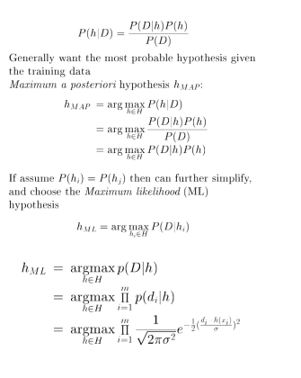
Looking at the last three equation, p(D/h) = p((d1, d2, d3)/h) can be reduced to multiplication only when d1, d2, d3 are independent.


Panel Data And Analysis

From Wikipedia

In statistics and econometrics, panel data or longitudinal data[1][2] are multi-dimensional data involving measurements over time. Panel data contain observations of multiple phenomena obtained over multiple time periods for the same firms or individuals

Time series and cross-sectional data can be thought of as special cases of panel data that are in one dimension only (one panel member or individual for the former, one time point for the latter).

A study that uses panel data is called a longitudinal study or panel study.


Cross sectional data:

Cross-sectional data, or a cross section of a study population, in statistics and econometrics is a type of data collected by observing many subjects (such as individuals, firms, countries, or regions) at the same point of time, or without regard to differences in time.

Analysis of cross-sectional data usually consists of comparing the differences among the subjects.


Examples


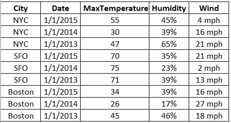
Panel Data

panel

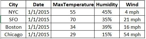
Cross Sectional Data

cs

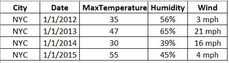
Time Series

ts

Regression Trees

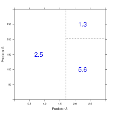
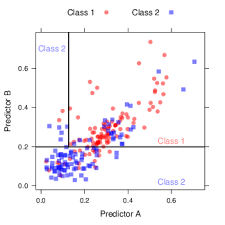
Figure below shows how decision tree creates rectangle in predictor space:

As we have describe classification tree, the only difference here is how to come up with output instead of label and how to define a metric other than entropy/gini.

For output it uses the mean of leaves.

For metric CART methodology uses simple SSE.

  • SSE = ∑ (y_i – y1)² + ∑(y_i – y2)²
    • where y1 and y2 are means of two newly crated groups.
    • It is simple sum of squares, not standard deviation 
    • While deriving R2 in linear recession we were concerned with sum of squares
    • Ward linkage criterion in hierarchical clustering also uses difference in sum of squares
  • diff = SSE_before – SSE_after
    • We choose a predictor which minimizes SSE the most.
    • diff is highest

My hand-coded regression tree is available at : https://github.com/arcarchit/datastories/tree/master/regression_tree

Reference

Applied predictive modeling by Max Kuhn and Kjell Johnson

Classification Trees

How classification Tree creates Rectangle in Predictor Space

Criterion for Choosing the Splitting Predictor

When deciding which predictor to split on, we need to consider different types of predictors: continuous, binary, and categorical. In this post, we will focus on continuous and binary predictors.

For categorical predictors, one approach is to use the “one vs rest” strategy. We evaluate each category separately and observe which one reduces the randomness the most when split.

In the case of a continuous predictor, we first sort the values and then select the midpoint as the split point.

To keep our decision tree simple, it’s ideal to have a small tree size. Therefore, at each step, we should choose the split that leads to the purest child nodes.

Two commonly used criteria for measuring impurity are Gini and Entropy. It’s important to note that these criteria are not directly used to select the predictor to split on. Instead, we calculate the difference in impurity before and after splitting.

When computing Gini or entropy after splitting, we apply weights to both splits to account for their proportions.

Multi-class

Decision tree can naturally handle multi class problem as entropy and gini can be calculated for multi-class.

Entropy

  • Formula:
    • H = ∑ -p * log(p)
  • About :
    • Randomness
    • Information Carries
    • Highest when p=0.5
    • Higher Entropy => Higher Randomness => Carries more information
    • After splitting we want entropy to reduce
  • Initial :
    • n0 positive and m0 negative sample
    • g0 = (n+m) total samples
  • After Splitting
    • Group 1:
      • n1 positive
      • m1 negative
      • g1 = (n1 + m1) total
    • Group 2:
      • n2 positive
      • m2 negative
      • g2 = (n2 + m2) total
  • Before Entropy :
    • H_before =  -(n0/g0) log(n0/g0) – (m0/g0)log(m0/g0)
  • After Entropy :
    • H1 = -(n1/g1) log(n1/g1) – (m1/g1)log(m1/g1)
    • H2 = -(n2/g2) log(n2/g2) – (m2/g2)log(m2/g2)
    • H_after = (g1/g0) * H1 + (g2/g0)*H2
  • diff = H_before – H_after
  • Select a predictor for which diff is highest and split on it
    • Which means we are selecting a predictor which reduces randomness more
    • Which also mean we are selecting a predictor which reduces information more
      • So we are selecting a variable which carries more information
        • More important feature

Gini

  • Gini for 2 class :
    • G = p1 * (1-p1) + p2 * (1 – p2)
    • Using (p1 + p2 = 1) we can derive that G = 2*p1*p2
  • Gini in general:
    • G = ∑ p * (1 – p) = 1 – ∑ p²
  • Like entropy gini is maximum when p1 = p2 = 0.5
    • In this case nodes are least pure
  • Gini is a measure of impurity which we want to reduce by splitting on predictor
  • diff = G_before – G_after
    • We will select a predictor for which diff is highest

Entropy vs Gini

  • Given a choice gini will be better as computing log is costlier.
  • Both of them are better than “classification error as metric” [1]
    • Which would be selecting majority class for calculating classification error
    • It is useful while pruning but not while growing the tree

ROC Curve

  • ROC curve can be constructed easily for classifier which outputs ranking.
  • On the contrary decision tree outputs label
  • However to get a ROC we can use workaround. Each leaf node will have some positive and negative samples and we can calculate probability as (# positive / # total).
  • Then we can change the threshold and plot ROC.

Regularization

Regularization in decision tree will be explained in separate blog in detail, but here is the list of candidate techniques.

  1. limit max. depth of trees
  2. Cost complexity pruning
  3. ensembles / bag more than just 1 tree
  4. set stricter stopping criterion on when to split a node further (e.g. min gain, number of samples etc.)

Reference

[0] : Applied predictive modeling by Max Kuhn and Kjell Johnson

[1] : https://github.com/rasbt/python-machine-learning-book/blob/master/faq/decision-tree-binary.md

Q-Learning

Value Function

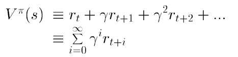
This represents value of a given state for the policy π.

q1

Optimal Policy

q2

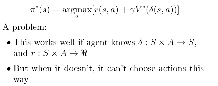
Learning Via Value Function is not possible when we don’t know immediate rewards and next state. If they are known we can use dynamic programming methods described at Dynamic Programming for RL.

q3

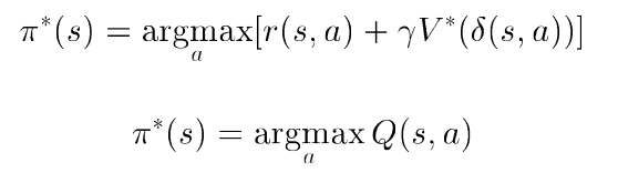
Q function

q41

q42

How it solve the problem of unknown reward and next state functions?

  • To calculate value function we need to know immediate reward for next state and probability of moving into next state
  • In Q learning we are don’t need them
    • We just take best action, then observe the reward for whichever state we go in.
    • It is possible to know reward after taking action, not before that.


Training Rule for Q

We initialize Q table with random values and keep updating it on each action based on reward get.

q5

We have trained grid world with above equation. Notebook is available at [2]. One thing to note in that code is that, we don’t need backup. We don’t need to update entire q table simultaneously. We can calculate new value for once cell and write it at once.

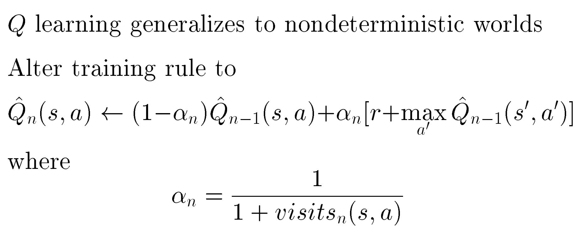
Also [1] is a very good resource. It shows changes in the Q-update equation in non deterministic world. (Reward and next state are non deterministic).

qq3

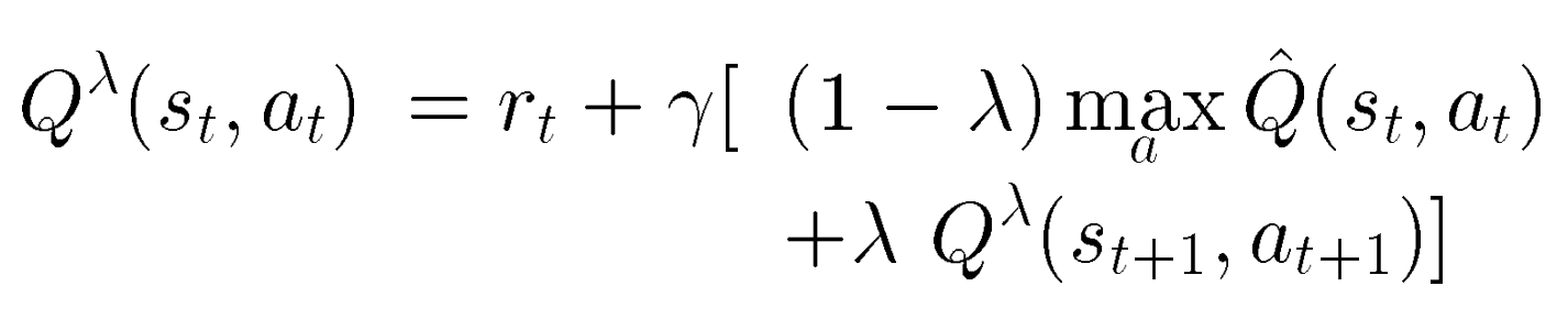
And also derives TD updates (Temporal Difference)

qq4


Convergence Conditions

  • System is deterministic MDP (Markov Decision Process)
  • Immediate reward values are bounded
  • Agent visit every state action pair infinitely often


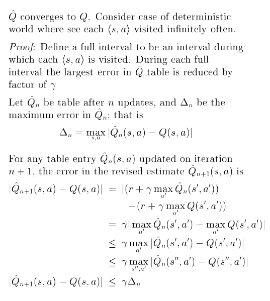
Derivation for Convergence

q6

Experimental Strategies

  • We also need to do exploration
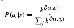
  • So we pick up action with a probability such that
    • action having more Q value has higher probability
  • One way to formulate this is as follows where in value of k control exploration-exploitation trade-off.
    • Initially k is small (exploration) and then is slowly increased (exploitation)

q7


How can we speed up Updating Sequence

  • Strategy 1
    • Consider the case for single absorbing goal state case. (What it means that if agent’s goal is to reach particular state) and initially all (q,a) pairs are initialized with 0.
    • So only one (q,a) pair will be update when we reach to reward state,
    • To speed up things, we can store intermediate state and action and then update backward till origin once we reach reward state.
    • Of course this will increase memory requirement
  • Strategy 2
    • Store immediate reward of past along with state-action pair and retrain periodically
    • If one Q(s, a) changes it will help change others as well
  • Strategy 3
    • If performing real environment action in environment is difficult we can perform simulation


Reference :

[0] Machine Learning by Tom Mitchell

[1] http://www.cs.cmu.edu/afs/cs.cmu.edu/project/theo-20/www/mlbook/ch13.pdf

[2] https://github.com/arcarchit/datastories/blob/master/RL_GridWorld.ipynb


Simple Linear Program

Purpose is to know how it looks solving linear programs using libraries and solvers.

Reference : https://pythonhosted.org/PuLP/CaseStudies/a_blending_problem.html


\* Minimize food cost *\
Minimize
Total_Cost: 0.008 Beef_percentage + 0.013 chicken_percentag
Subject To
Fat_Constraint: 0.1 Beef_percentage + 0.08 chicken_percentag >= 6
Fiber_Constrint: 0.005 Beef_percentage + 0.001 chicken_percentag <= 2
Protine_Constraint: 0.2 Beef_percentage + 0.1 chicken_percentag >= 8
Salt_constraint: 0.005 Beef_percentage + 0.002 chicken_percentag <= 0.4
Total_Sum: Beef_percentage + chicken_percentag = 100
End


"""
THis is taken from https://pythonhosted.org/PuLP/CaseStudies/a_blending_problem.html
"""
from pulp import *
problem = LpProblem("Minimize food cost", LpMinimize)
x1 = LpVariable("chicken_percentag", lowBound=0)
x2 = LpVariable("Beef_percentage", lowBound=0, upBound=None)
problem += 0.013*x1 + 0.008*x2, "Total Cost"
problem += x1 + x2 == 100, "Total Sum"
problem += 0.1*x1 + 0.2*x2 >=8, "Protine Constraint"
problem += 0.08*x1 + 0.1*x2 >=6, "Fat Constraint"
problem += 0.001*x1 + 0.005*x2 <=2, "Fiber Constrint"
problem += 0.002*x1 + 0.005*x2 <=0.4, "Salt constraint"
problem.writeLP("minimize_food_cost.lp")
problem.solve()
print "Solution found was :", LpStatus[problem.status]
print "Here is the proportional of chick and beef that should be used"
for v in problem.variables():
print "\t",v.name, " : ", v.varValue
print "Cost will be : ", value(problem.objective)

view raw

pulp_LP.py

hosted with ❤ by GitHub


Solution found was : Optimal
Here is the proportional of chick and beef that should be used
Beef_percentage : 66.666667
chicken_percentag : 33.333333
Cost will be : 0.966666665

view raw

std_output.txt

hosted with ❤ by GitHub


ARIMA model

ARMA to ARIMA

  • When there is a trend in data we take differences
  • ARIMA – Auto regressive Integrated Moving average
  • Integrated term includes order of difference, In the example below it is d=2

arima

Below is the sample github gist and output pdf is avaialble at ARIMA model.pdf


—
title: "ARIMA model"
author: "Archit Vora"
date: "April 3, 2018"
output: html_document
—
“`{r setup, include=FALSE}
knitr::opts_chunk$set(echo = TRUE)
“`
We will try to fit ARIMA model to BJsales dataset from 'dataset' package in R.
Here is the plot of it.
“`{r}
library(datasets)
plot(BJsales)
“`
Mean in changing over time and seems time series is not statioary. Let's take the difference.
“`{r}
plot(diff(BJsales))
“`
Seems It is still not staionary, let's take one more diff.
“`{r}
plot(diff(diff(BJsales)))
“`
Now it seems stationary. Let's plot acf and pacf of this doubly differenced series.
“`{r}
focus<- diff(diff(BJsales))
acf(focus)
pacf(focus)
“`
From ACF lag 1, 8 and 11 seems significant, while from PACF seems lag 1, 2, 3, 10 and 19 seems significant.
Keeping parsimonious principle in mind we shall consider order of 0 and 1 for MA terms and oreder of (0, 1, 2, 3) for AR terms.
Now let's try differenct models and check their AIC.
“`{r}
d <- 2
for (p in 0:3){
for (q in 0:1){
if(p+d+q<6){ # Ensures simple model
mm<- arima(x = BJsales, order = c(p, d, q))
pval <- Box.test(mm$residuals, lag = log(length(mm$residuals)))
sse <- sum(mm$residuals^2)
aic <- mm$aic
cat(p, d, q, "AIC = ", aic, "SSE = ", sse, "P-value = ", pval$p.value, "\n")
}
}
}
“`
Seems like (0, 2, 1) has smallest AIC but does not have significant p-value.
Let's leave it for this post and plots residual.
“`{r}
model <- arima(x = BJsales, order = c(0, 2, 1))
par(mfrow = c(2, 2))
plot(model$residuals)
acf(model$residuals)
pacf(model$residuals)
qqnorm(model$residuals)
“`
There seems no significant correlation as well as QQ-plot also looks okay.
Now let's plot the forecast.
“`{r}
library(forecast)
fc <- forecast(model, h=20)
plot(fc)
“`
All this can also be done by auto.arima routine of forecast package.
“`{r}
model <- auto.arima(BJsales, seasonal = FALSE)
model
fc <- forecast(model, h = 20)
plot(fc)
“`
auto.arima has come up with different model, but it is okay.

view raw

arima.Rmd

hosted with ❤ by GitHub

Fitting AR Processes

Yule Walker Equation in Matrix Form


ym1

  • If we write and above equation for k=1, 2, . . ., n and use the fact that ρ(k) = ρ(-k), we can write it in a matrix form.
  • Using the data we have we can estimate values of ρ  (auto correlation coefficients)
  • acf() routine in R gives us that
  • Using values of ρ we can then estimate values of Φ (parameters of AR process)


ym2

  • Above is an example for AR process
  • We can solve these equation for values of Φ1, Φ2 and Φ3


Reference:

Moving average and Auto-regressive Processes

Moving Average Processes MA(q)

  • Stock price depends on announcements of last two days
  • Auto correlation function cuts off at q

maq


Auto regressive Processes AR(p)


1

2

3


  • Below are the plots for AR(2) process
  • Depending upon the value of phi1 and phi2 ACF has alternative positive and negative values


56


Writing AR(p) process as MA process by substituting values of X(t-1). And yes phi is constant, we don’t need phi1, phi2 anymore.

78


Mean, variance and auto-correlation of AR(p) process, we have assumed Z = Norm(0, sigma2)

9


ACF of AR-p using Yule-Walker Equation

  • It is a method of solving difference equation in recursive relation
  • We first obtained auxiliary equation (also known as characteristic equation) which is polynomial and find root of that
  • Using these root we get weighted geometric series and find weights using some initial condition
  • We had learned in mathematics that this way of solving difference equation also related to solving differential equations
  • In the course they had solved it for Fibonacci series and root had come out to be golden ratio
  • For AR(p) ACF comes out to be difference equation, solving which can give us ACF for different values of lag


Reference

https://www.coursera.org/learn/practical-time-series-analysis/home/welcome

https://en.wikipedia.org/wiki/Autoregressive%E2%80%93moving-average_model