On Classification Accuracy – 2

We have already talked about it in this post. Just want to add few more things after finishing a course. This post is just an extension of above with some practical considerations.

We are claiming that accuracy may not be a good measure always. When you are building automated machine learning you must trust it.

Case Study

  • You want to show positive reviews on your website.
  • Say in your dataset 90% reviews are negative.
  • A classifier can achieve 90% accuracy by predicting all of them as negative.
  • But what you are interested in is finding out remaining 10% and display it on your website.


Precision = Did I show something negative?

Recall = How good I am at finding positive reviews?


Analogy with Optimist and Pessimist

  • Optimist assigns every/most review as positive
    • Very good recall, but less precision
  • Pessimist assigns every/most review with negative
    • Bad recall, good precision


Trade-off

  • Trade-off comes while scoring, not while training
  • We can assign labels based on probabilities
  • Decision tree gives probability by no of positive and negative samples at leaf node
  • Logistic regression of-course gives probability
  • We can change threshold to trade off between precision and recall
  • Positive when prob > 1 => Pessimist
  • Positive when prob > 0 => Optimist


Single no not always useful

  • Single numbers like F1 score and AUC are something I am not great fan of
  • You can not always choose classifier just by AUC, ROC curve might intersesct
    • This intersection means that one classifier is better at some range of precision
    • But if they don’t intersect we choose the one with higher AUC
  • From business perspective we are should be clear whether we want more precision or recall
  • Another practical metric they talked about was precision at k
    • Say I want to display 5 reviews on my website
    • What is the precision after 5 values I have chosen


When to use different metrics ?

Pick the metric that matches what the model’s output is consumed by.

A retrieval layer emits a ranked list under a budget → only the ordering matters → AUC / recall@k. 

Topic classification emits a hard label → you’re evaluating cells of a confusion matrix → F1.

CTR emits a probability that gets multiplied by something downstream (bid = pCTR × value) → being off by 2x in the probability directly costs money even if the ranking is perfect → you need a calibration-sensitive metric → NE.

1. Threshold / confusion-matrix metrics (output is a decision)

  • Accuracy — nearly useless under imbalance
  • Precision, Recall, Specificity (TNR), FPR
  • F1; F-beta (β>1 favors recall, β<1 favors precision)
  • Macro vs micro vs weighted F1 — macro treats every class equally so rare topics actually show up; micro is dominated by head classes. For topic classification this choice usually matters more than F1 vs anything else.

2. Ranking / threshold-free metrics (output is an ordering)

  • ROC-AUC — P(random positive scores above random negative). Invariant to any monotone rescaling, which is exactly why it can’t catch a miscalibrated CTR model.
  • PR-AUC / Average Precision — the one you want under heavy imbalance. ROC-AUC’s baseline is 0.5 regardless of prevalence; PR-AUC’s baseline is the prevalence, so it doesn’t flatter a model on a 0.1% positive rate.
  • Gini = 2·AUC − 1; KS statistic (max gap between the two score CDFs) — both standard in credit risk
  • NDCG, MRR, MAP when relevance is graded rather than binary

3. Probabilistic / calibration metrics (output is a number you do arithmetic on)

  • Log loss — proper scoring rule, penalizes both discrimination and miscalibration
  • NE = log loss ÷ entropy of the empirical base rate. The normalization is what makes it comparable across surfaces, countries, and time periods with different base CTRs; 1.0 = no better than always predicting the base rate.
  • Calibration ratio / COPC (sum of actuals ÷ sum of predictions) — the bias check that NE alone won’t give you cleanly

Step Size in Descent Methods

Descent Method

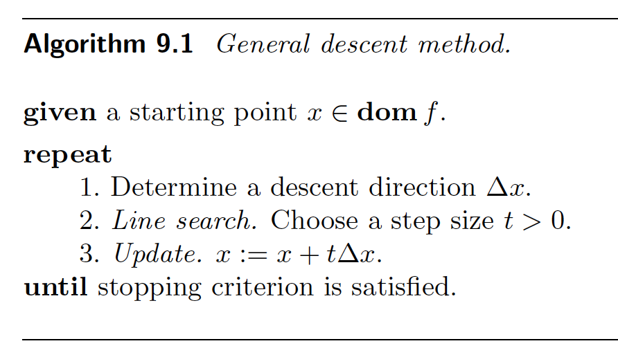
general_descent

  • When the descent direction is opposite to gradient is is called gradient descent.
  • We also have steepest descent and newton’s algorithm
  • In this post we will focus on line search
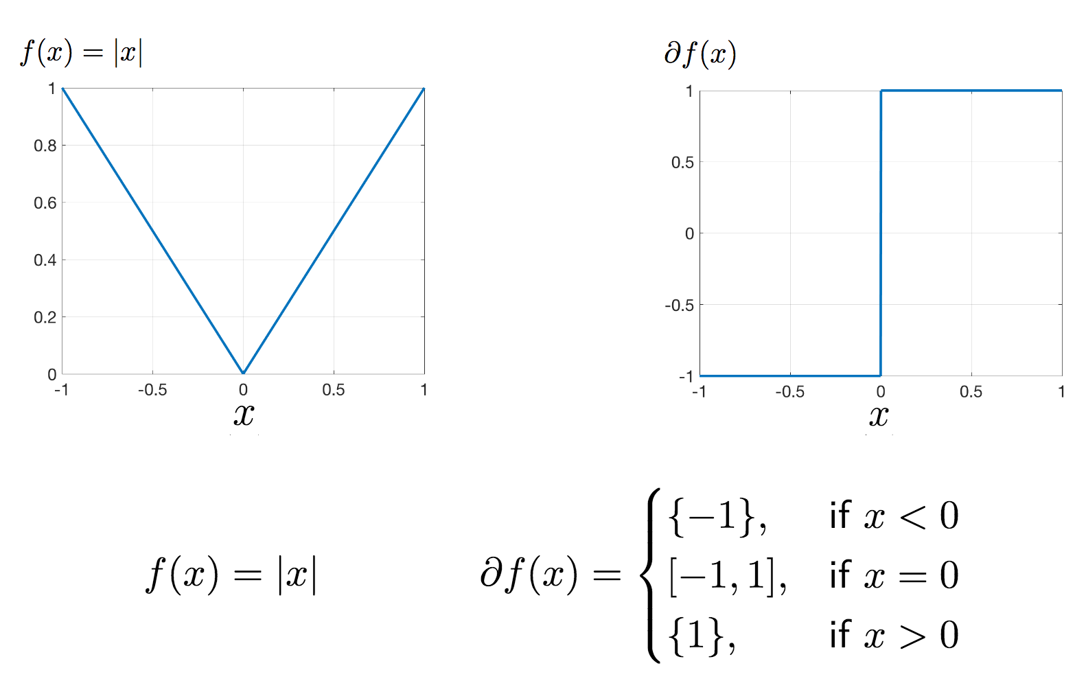
  • Term is called ‘line search’ because step size t determines where along the line {x + t ∇ x } next iterate will be. (ray search would be more appropriate term)


Fixed Step Size

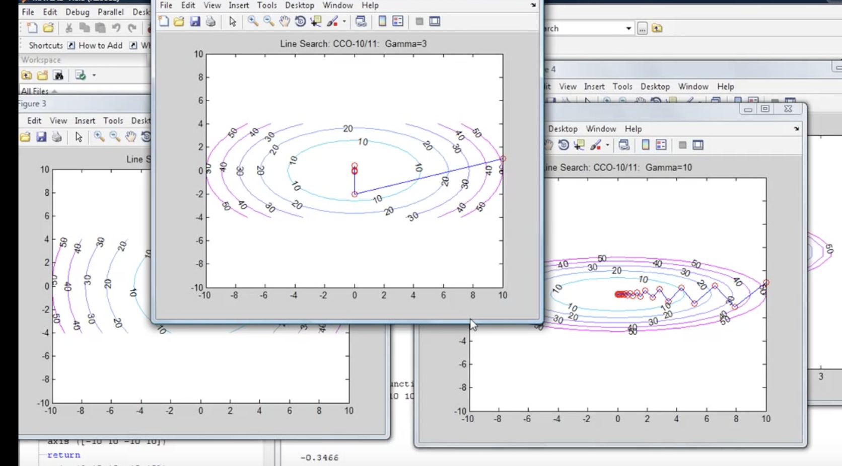
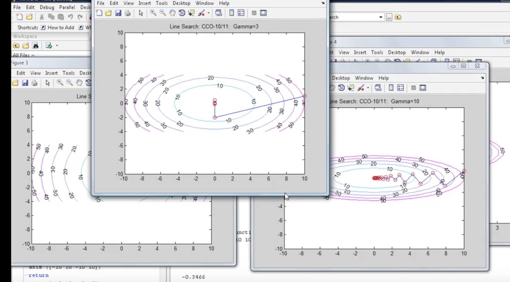
  • Here we keep the step size (t) constant for all the iteration
  • Our solution many not converge if t is too large
  • If can take a lot of time if t is too small


faster_iteration


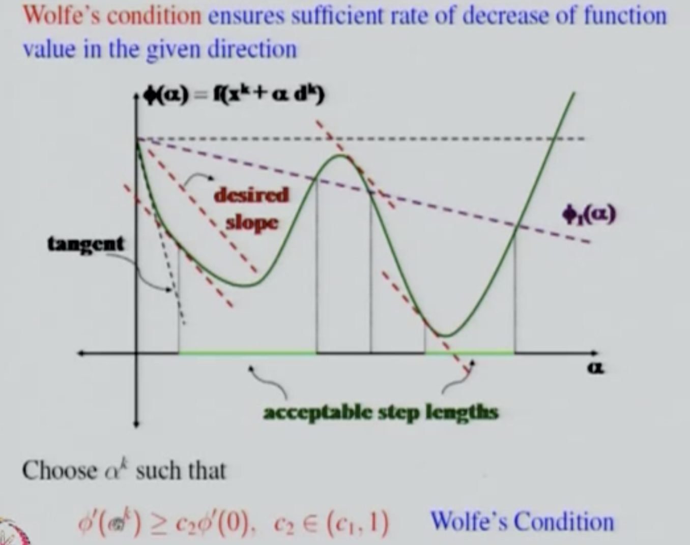
Exact line search

exact_line_search

  • It is used when cost of minimizing problem with one variable (s) is less than computing direction (∇ x)


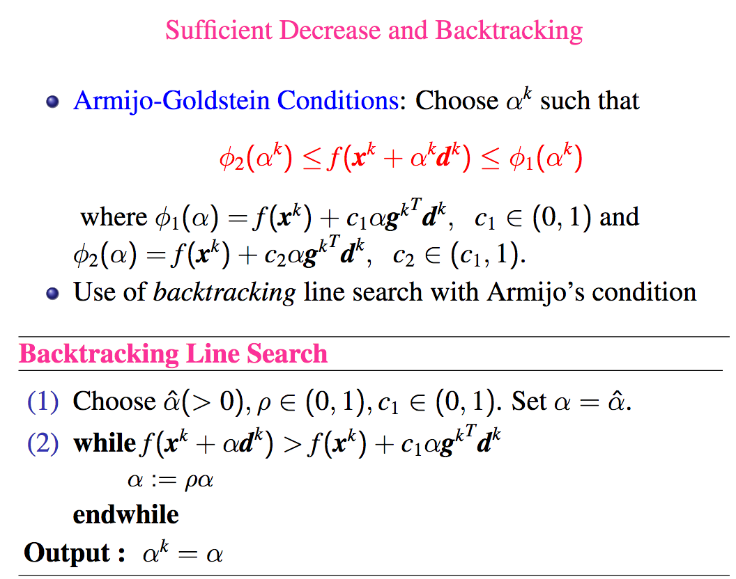
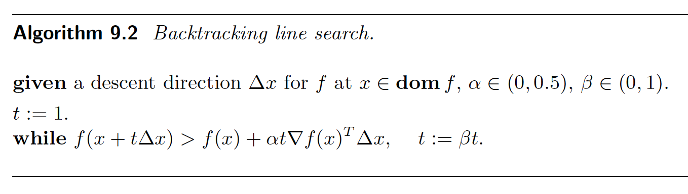
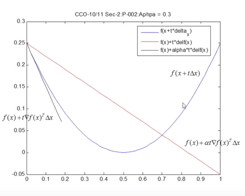
Backtracking Line Search

  • Exact line search has to solve optimization problem and become computational inefficient
  • This is most widely used in practice.
  • Here we don’t find optimal value of t, but some approximation

inexact_line_searchonethreetwo


Demo of Convergence


faster_iteration


References


knn and kernel regression

This is to summarize learning from course by University of Washington hosted on Coursera.


Parametric vs Non parametric

Parametric models have a predefined complexity, meaning the complexity is fixed regardless of the number of observations. On the other hand, non-parametric models allow the complexity to grow as the number of observations increases.

Infinite Noiseless Data

When dealing with infinite noiseless data, it is important to note that quadratic fit introduces some bias. However, 1-NN (nearest neighbor) can achieve zero RMSE (root mean squared error).

Examples of Non-parametric Models

Non-parametric models include kNN (k-nearest neighbors), kernel regression, spline, and trees. These models do not make strong assumptions about the underlying data distribution and can adapt to varying complexities based on the observed data.

1 NN

n the nearest neighbor (NN) prediction, we identify the closest data point to the query point, and the response of that nearest point is considered as our prediction.

Voronoi Tesselation

When working with multidimensional data, plotting the nearest neighbor prediction results in a Voronoi tesselation, also known as a Voronoi diagram. This diagram divides the space into regions based on the closest data point for each query point.

Distance Metrics

Distance metrics play a crucial role in nearest neighbor algorithms. Some commonly used distance metrics include:

  • Euclidean distance: Measures the straight-line distance between two points in the feature space.
  • Scaled Euclidean distance: Allows for different weights on different dimensions, which is useful when certain features carry more importance. For example, in predicting house prices, the square footage may be weighted more heavily than the number of floors.
  • Other examples of distance metrics include Mahalanobis distance, rank-based distance, correlation-based distance, cosine similarity, Manhattan distance, and Hamming distance.

1 NN in Practice

The 1 NN algorithm performs well when the data is dense. However, there are limitations to its effectiveness:

  • In non-dense data regions, it struggles with interpolating between observations.
  • It is sensitive to noise, as a single noisy data point can significantly impact the prediction.
  • 1 NN tends to overfit the training data, resulting in poor generalization to new observations.

To address these limitations, the k-nearest neighbors (kNN) algorithm is often employed.


k-Nearest Neighbors (kNN)

In the kNN algorithm, we consider the k nearest neighbors and use their responses as predictions. This approach helps reduce the impact of noise compared to using only the nearest neighbor (1NN).

Challenges:

  1. Boundary issues: When dealing with boundaries, the same points may repeatedly appear as nearest neighbors, resulting in a flat response.
  2. Sparse region issues: In sparse regions, the same points may also be repeatedly chosen as neighbors, leading to potential inaccuracies.
  3. Discontinuity of fit: The fit obtained using kNN may not be smooth since one neighbor can suddenly be excluded from the set of nearest neighbors.

To address these challenges, we can employ weighted kNN, which assigns different weights to each neighbor based on their proximity.

Weighted k-Nearest Neighbors (kNN):

In weighted kNN, less weight is assigned to neighbors that are farther away from the query point. This approach helps mitigate the issue of fit discontinuity in standard kNN.

There are two common weighing schemes used in weighted kNN:

  1. Simple weighing scheme: In this scheme, the weight assigned to each neighbor is inversely proportional to its distance from the query point. The formula for weight calculation is: weight = 1 / distance.
  2. Sophisticated weighing scheme using kernels: Kernels, such as the Gaussian kernel, are employed to assign weights. The Gaussian kernel never reaches zero, ensuring that even distant neighbors have some influence. On the other hand, kernels like the Uniform or triangular kernel eventually reach zero, diminishing the influence of distant points. The parameter λ is used to control how quickly the kernel reaches zero. A faster decay indicates that distant points will have less influence.

By incorporating weighting schemes in kNN, we can achieve a more nuanced and smoother fit, addressing the issue of fit discontinuity encountered in standard kNN.

Kernel Regression:

Kernel regression is an alternative approach to kNN, where instead of considering only k neighbors, we consider all observations in the dataset. This allows for a more continuous and smoother prediction.

The choice of kernel in kernel regression can be either bounded, such as the uniform or triangular kernel. In such cases, we consider a subset of neighbors, but it is not strictly a kNN approach.

When performing kernel regression, two decisions need to be made:

  1. Choice of kernel: The choice of kernel has a relatively smaller impact on the prediction. Various kernels can be used, and their selection is typically based on the specific problem at hand.
  2. Choice of bandwidth: The bandwidth plays a more significant role in the prediction. It determines the spread of the kernel before it reaches zero. A small bandwidth can lead to overfitting, capturing noise and local fluctuations, while a large bandwidth can result in an overly smoothed fit, leading to high bias. The bandwidth can be tuned using the kernel’s parameter λ, which can be selected through techniques such as cross-validation.

By considering all observations and utilizing kernels in kernel regression, we can achieve a more flexible and continuous prediction model, providing a trade-off between bias and variance based on the choice of bandwidth.

Local Linear Regression

Up until now, we have discussed the use of weighted averages for prediction. However, an alternative approach is to fit a model in the vicinity of the prediction point, where the errors are weighted by a kernel.

In local linear regression, we can fit either a linear model or a quadratic model near the prediction point. A linear model is particularly useful for addressing boundary effects, as it provides a linear prediction instead of a constant one.

On the other hand, a quadratic fit can handle curvature in the data but may introduce higher variance in the predictions. Consequently, in practice, a linear fit is often recommended due to its favorable balance between bias and variance.

By employing local linear regression, we can adapt the model’s behavior based on the local data characteristics, enabling more accurate predictions near the prediction point.

Global vs Local Fit

In certain situations, we may find that a linear fit is appropriate for some regions of the input space, while a quadratic fit is more suitable for others. However, determining the breakpoints where the underlying structure changes can be challenging.

Non-parametric models come to the rescue in such cases. Instead of assuming a specific functional form, these models allow for more flexibility in capturing the underlying patterns.

One example of a global fit is taking the average as a constant prediction. This approach provides a simple representation of the data but assumes a uniform behavior across all observations.

On the other hand, kernel regression offers a way to achieve a local fit by applying different weights to each observation. Nearer observations receive higher weights, enabling the model to adapt to local variations in the data.

By leveraging non-parametric models like kernel regression, we can capture both global and local characteristics of the data, allowing for more accurate and adaptive predictions based on the proximity of observations.

Limitations of Non-parametric Approaches

While non-parametric approaches like kNN offer flexibility and adaptability, they do have certain limitations.

  1. Dimensionality: In higher dimensions, non-parametric models require an exponentially large number of observations to accurately capture the underlying patterns. As the number of dimensions increases, the data becomes more sparse, making it challenging to find sufficient neighboring points for accurate predictions.
  2. Data Availability: Non-parametric models heavily rely on the availability of a large amount of data. When the dataset is limited or scarce, it becomes difficult to leverage the full potential of non-parametric approaches.
  3. Computational Complexity: Non-parametric models, such as kNN, involve a brute force search to find the nearest neighbors. This search operation has a complexity of O(N) for 1-NN and O(N log K) for k-NN, where N is the number of observations. While these complexities can be manageable for smaller datasets, they can become computationally expensive as the dataset grows larger.

To mitigate some of these limitations, techniques like clustering can be employed to reduce the search space and improve computational efficiency.

In situations where the dataset is limited or high-dimensional, parametric models offer an alternative by making certain assumptions about the underlying structure. These models provide a more compact representation and are often more suitable when data availability or computational complexity is a concern.

Understanding the limitations of non-parametric approaches helps in selecting the most appropriate modeling technique based on the specific characteristics of the dataset and the available resources.

References

Course by University of Washington

https://www.coursera.org/learn/ml-regression



Generalized Linear Models (GLM)

In standard linear regression we make two assumption :

  1. P(Y/X) is a normal distribution
  2. Mean is a linear function of parameter µ  = β*X
  3. P(Y/X) = Ν(µ, σ^2* I)       # σ is standard deviation and I is identity matrix


In GLM we relax two things :

  1. P(Y/X) is from any exponential family
  2. Mean is some function of β*X
    1. µ = f(β*X)
    2. g(µ) = β*X
    3. g = f^(-1)
    4. g is called link function


Example of link functions:

  1. log link
  2. reciprocal link
  3. logistic link


Derivation of log-likelihood matches that of normal distribution. However closed form solution is not defined and is generally solved by least square and convex optimization.

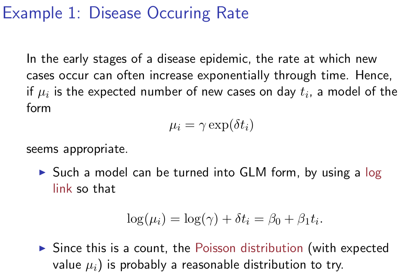
Here is one example from MIT course mentioned in references.

poisson

Logistic

  • In gaussian regression we predict μ for each sample
    • This μ comes from β0, β1, β2 which are same for each sample
  • For binomial regression we want to predict p for each sample
    • This p comes from β0, β1, β2 which are same for each sample
  • One option :
    • p = β0 + β1*x1 + β2*x2
  • Second option
    • p = sigmoid (β0 + β1*x1 + β2*x2)
    • f(p) = log(p/(1-p)) = β0 + β1*x1 + β2*x2
    • It is logit link function
  • What are other options apart from sigmoid
    • step function (Not differentiable, that is why we use (sigmoid)
    • tanh is sometime used in deep learning
  • What if we go with option 1:
    • Binomial distribution requires p to be in (0,1)
  • Example :
    • How many fishes survive (alive/dead) given food and water


Poisson

  • Poisson distribution models probability of observing count


      • P(k) = exp(-λ) * (λ^k) / k !


    Parameter λ >= 0

  • Option one:
    • λ = β0 + β1*x1 + β2*x2
  • Option two:
    • λ = exp ( β0 + β1*x1 + β2*x2 )
    • f ( λ ) = log ( λ ) = ( β0 + β1*x1 + β2*x2 )
    • It is log link function
  • What if we go with option one:
    • We want λ > 0
    • Relationship between input and output is not additive but multiplicative ?
      • Suppose the seeds have germinated as many as 1.5 times by the enough water and as many as 1.2 times by the enough fertilizer. When you give both enough water and enough fertilizer, the seeds would germinate as many as 1.5 + 1.2 = 2.7 times ?

        Of course, it’s not. The estimated value would be 1.5 * 1.2 = 1.8 times. [3]
  • Example:
    • How many seed will germinate given water and fertilizer


Parameter Estimation

  • We can do maximum likelihood estimate and find parameters β0, β1, β2
  • Deriving maximum likelihood for binomial:
    • max_lh = Multiply (Likelihood of y_acutal of each sample for predicted distribution)
    • max_lh = Multiply ( Binomial(p) )
    • max_lh = Multiply ( p if y=1 else (1-p) )
    • log(max_lh) = Summation (y*logp + (1-y) log (1-p))
  • Deriving maximum likelihood for Poisson:
    • max_lh = Multiply (Likelihood of y_acutal of each sample for predicted distribution)
    • max_lh = Multiply ( Poisson (u) )
    • max_lh = Multiply (exp(-u) * u^y / y! )
    • log(max_lh) = summation ( -u + y*log(u) – log (y!) )
  • Above two are rough derivations but conveys the idea
  • For Gaussian it turns out to OLS (Ordinary Least Squares) and has closed form solution
  • For other we solve it via gradient/newton’s method.

Why the gradient is the same for linear and logistic regression

If you write gradient descent for linear regression and then for logistic regression, you end up typing the same line twice:

grad = X.T @ (y_pred - y) / n

That is not a coincidence or a happy accident of notation. It is a theorem, and it explains a design decision that shows up throughout deep learning.

The pattern

ModelPredictionGradient
Linearŷ = XwXT(ŷ − y)
Logisticŷ = σ(Xw)XT(ŷ − y)
SoftmaxŶ = softmax(XW)XT(Ŷ − Y)
Poissonŷ = eXwXT(ŷ − y)

Identical in every case: XT × (prediction − target).

Why: the cancellation

Apply the chain rule to logistic regression and watch what happens. With z = Xw and p = σ(z):

∂L/∂w = (∂L/∂p) · (∂p/∂z) · (∂z/∂w)

The two middle terms are:

∂L/∂p = (p − y) / [p(1 − p)]      ∂p/∂z = p(1 − p)

The p(1 − p) cancels exactly. What survives is (p − y) · X, and the transpose assembles it into XT(p − y).

For linear regression there is nothing to cancel. The link is the identity, so ∂ŷ/∂z = 1 and you get the same form trivially.

The general statement

This is the canonical link property of generalized linear models. For any exponential-family likelihood

p(y | θ) = h(y) · exp( θy − A(θ) )

the mean is μ = A′(θ) and the variance is A″(θ). When you use the canonical link — meaning you set θ = Xw directly — the score function is always

∇w ℓ = XT(y − μ)

The curvature term A″ that the chain rule produces is exactly the same A″ sitting in the denominator of the loss derivative. It cancels by construction, because the link and the loss are both derived from the same log-partition function A(θ).

  • Linear → Gaussian, A(θ) = θ2/2, identity link
  • Logistic → Bernoulli, A(θ) = log(1 + eθ), logit link
  • Poisson → A(θ) = eθ, log link

One object, three instances.

Where it breaks, and why that matters

Pair a sigmoid with MSE instead of log-loss and the cancellation fails:

∇w = XT [ (p − y) · p(1 − p) ]

The extra p(1 − p) survives, and it is near zero whenever p is near 0 or 1. Measured on a small synthetic dataset at a weight vector where many predictions are confidently wrong:

log-loss gradient norm: 0.770
MSE gradient norm: 0.014

Fifty-five times smaller, in exactly the regime where the largest correction is needed. The model is badly wrong and the gradient says “barely move.”

That is the vanishing gradient problem in its simplest form, and it is why cross-entropy replaced squared error for classification. MSE paired with a sigmoid is also non-convex in w, so it has local minima; log-loss is convex.

It still converges on easy data — 200,000 iterations reached a negative log-likelihood of 0.3100 against log-loss’s 0.3098 in 1,000 — but that is roughly 200 times slower on a trivial problem. On anything harder it simply stalls.

The short version

The gradient is XT(prediction − target) for any GLM paired with its canonical link, because the link’s derivative cancels the loss derivative — both come from the same log-partition function. That is not a convenience. It is the reason those particular loss and activation pairs became the standard ones.


References :

[0] https://ocw.mit.edu/courses/mathematics/18-650-statistics-for-applications-fall-2016/lecture-slides/MIT18_650F16_GLM.pdf

[1] Wonderful MIT lecture : https://www.youtube.com/watch?v=X-ix97pw0xY

[2] https://onlinecourses.science.psu.edu/stat504/node/216/

[3] https://tsmatz.wordpress.com/2017/08/30/glm-regression-logistic-poisson-gaussian-gamma-tutorial-with-r/


Exponential Family

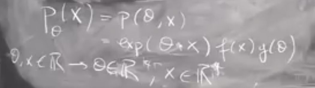
Here is the basic concept :

simple_exponential

  • θ are parameters and X is data, both can be multidimensional
  • We want to restrict terms inside exponential to the form θ*X


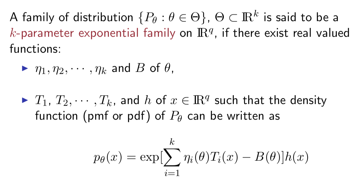
Formal Definition:

formal_defination

  • η and T functions also help for the case when there is a mismatch in the dimension of θ and X.
  • g(θ) in basic concept above has been taken into exponential as B(θ).
    • It vaguely serves as normalization factor.
  • h(x) serves a distribution and exponential transfer this basic distribution


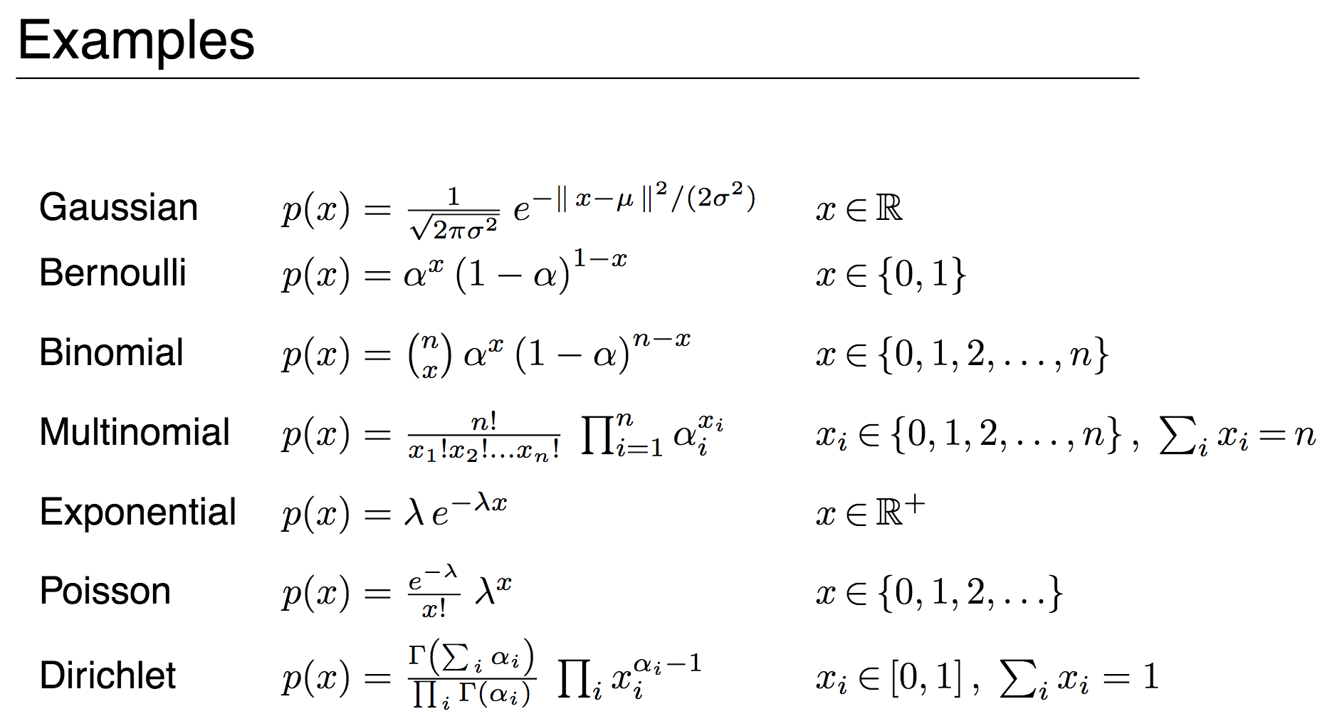
examples


Further Reading

Click to access chapter8.pdf

Click to access lecture12.pdf


Interpretation of Multiple Regression Coefficients

  • In case of simple linear regression with one variable we interpret slop coefficient as follows
    • y = b0*x0 + c
    • b0 is increase in y for unit increase in x0
  • In case of multiple regression:
    • y = b0*x0 + b1*x1 + c
    • b0 is increase in y for unit increase in x0 keeping x1 constant


Implication of keeping other variable constant:

  • Consider
    • house_price = b0 * no_of_bedrooms + c       ….. (1)
    • house_price = b0 * no_of_bedrooms + b1*square_feet + c     …..(2)
  • In (1) there are high chances that b0 will be positive
  • In (2) it can be negative
    • If you increase no of bedrooms keeping square feet constant each room will be smaller
    • This may decrease house price


Reference :

Coursera course on regression by University of Washington DC : https://www.coursera.org/specializations/machine-learning


Grubb’s Test for Anomaly Detection

Problem Statement:

We are receiving time series of count data everyday and we want to detect whenever there is drastic change in this count.


Grubb’s test assumes a t-distribution of input and find out the outliers for required confidence interval. We remove this outlier and repeat the test again. Here is the pseudo code:


Grubbs Test(X, p-val=0.05):
    Repeat :
        Z <- zscore(X)
        n < len(X)
        zi, index <- max(abs(Z)), index(max(abs(Z)))
        if zi > threshold(N, p-val):
            remove X[index] 
        else:
            break


Traditionally Grubb’s tests has a alternate hypothesis that exactly one outlier is present in data. In above we modified it get all possible outliers.


Test Hypothesis
Grubb’s Test H0: There are no outliers in the data set
Ha: There is exactly one outlier in the data
Tietjen-Moore test H0: There are no outliers in the data set
Ha: There are exactly k outliers
Generalized ESD test H0: There are no outliers in the data set
Ha: There are up to r outliers


Above can be extended to two sided tests as well.


We had followed this in time series based anomaly detection and following approach were considered for pre processing before applying Grubb’s test:

  • Raw Count (No processing)
  • Residuals after STL decomposition
  • Residuals after fitting ARIMA

In our case raw count had worked well enough.


Reference:

https://www.itl.nist.gov/div898/handbook/eda/section3/eda35h1.htm

Github Gist


Ensemble, Bagging and Boosting

Ensembling is a method of combining more than one models to generate a final output.(Reference [1])

There are two ways of doing that:

  1. Bagging
  2. Boosting


Bagging Boosting
  • We take subset of data and train different models
  • Example Random forest
    • It takes subset of data as well as subset of features
  • Pros of random forest
    • Handles high dimensions
    • Handles missing values
  • Cons of random forest
    • It won’t give precise value regression because final value is mean from subset tress
    • None the less people are using it for regression depending upon domain
  • We train different model on with same data. Each sample is assigned different weight in each iteration
  • Example AdaBoost, XgBoost
  • Pros of XgBoost
    • Supports different loss function
    • Works well with interactions
  • Cons of XbBoost
    • Prone to overfitting
    • Tuning of hyper parameters is critical


Pros-cons of bagging vs boosting:

  • Bagging is easy to parallelize and hence training is faster
  • Boosting is more efficient for fixed no of iterations (classifiers)


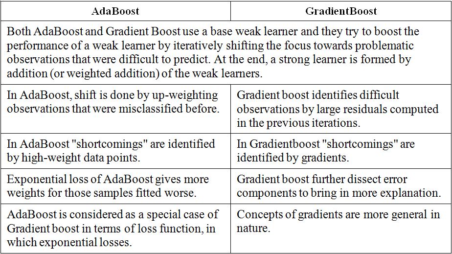
AdaBoost vs XgBoost

Reference : [2]

ada_vs_xg

Quote from Tianqi Chen, one of the developers of XGBoost:

Adaboost and gradboosting [XGBoost] are two different ways to derive boosters. Both are generic. I like gradboosting better because it works for generic loss functions, while adaboost is derived mainly for classification with exponential loss.


Reference :

[1] https://towardsdatascience.com/decision-tree-ensembles-bagging-and-boosting-266a8ba60fd9

[2] https://www.packtpub.com/mapt/book/big_data_and_business_intelligence/9781788295758/4/ch04lvl1sec34/comparison-between-adaboosting-versus-gradient-boosting


AdaBoost

  • AdaBoost stands for adaptive boosting
  • Boosting is a technique for creating better classifier form several regular/weak/base classifiers
  • Thought:
    • We want to train second classifier in such a way that training data has more samples for the case where first classifier was wrong
    • Third classifier will have more samples where first and second classifier contradicts
  • How do we accomplish above:
    • We assign weights to each sample
      • This weights will be used in error function for each sample
      • Error function would be sum of weights of incorrectly classified samples
      • This weights keep changing in each iteration
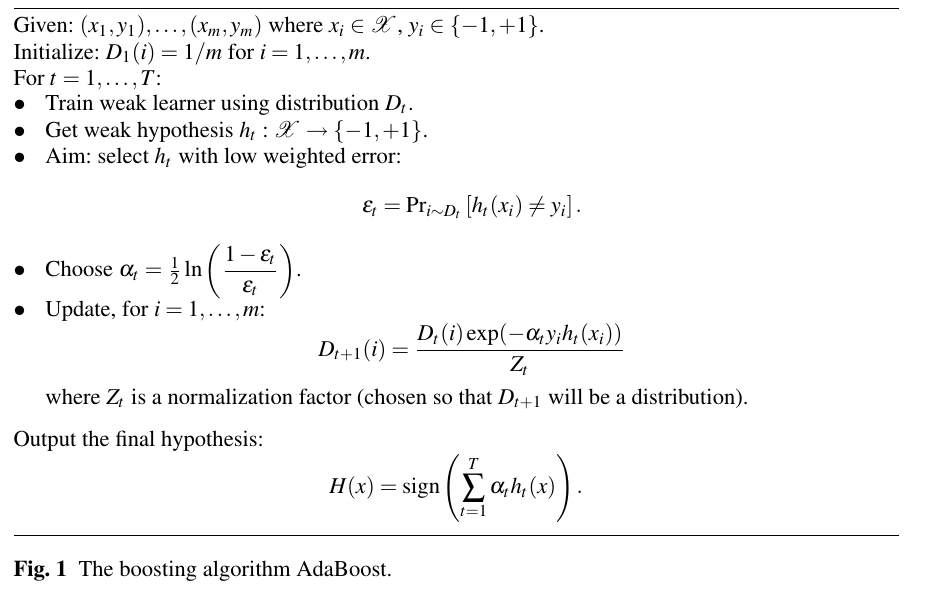
    • We also assign wight to each base (weak) classifier (α In below algorithm)
      • Formula for calculating α below is valid for binary classification
        • It will be different for multi class classification
  • When do we stop iteration ?
    • Combined classifier is predicting all sample correctly
    • No more base classifier left
  • Most machine learning algorithms allows to apply weight to data
    • In logistic regression we can multiply weight in error fucntion
    • In decision tree, classification error can be calculated by summing weights of missclassified samples


adboost


Formulations in above algorithm:

  • Formula of α
    • if ε=0.5 then α=0. It is just a random chance classifier.
    • Else it can positive/negative.
    • ε < 0.5 => negative α => we invert the prediction in weighted average
  • Formula of D_(t+1)(i)
    • y*h is just a sign
      • y and h are  {-1, 1}
      • y*h will be positive for correct prediction
    • Why it is function of ε
      • Random classifier updating weights does not make sense
  • By Z_t we are normalizing weights, which ensures numerical stability


Adaboost Theorem

  • Error -> 0 as no of iteration -> infinity at certain condition
  • Condition is here is that each learner has error < 0.5
  • Each iteration means adding one weak learner


Over-fitting

  • Contrary to weak classifier (decision stumps) we saw that rate of increase test error is less with boosting
  • However no of iteration still should be selected via cross validation for small data-set and validation for large data-set


References:

Click to access MIT6_034F10_boosting.pdf

Click to access msri.pdf