We rarely heard of nonparametric tests while reading standard statistical books. However there are some scenarios where they should be used instead of parametric tests. [1] has beautiful blog about it, I am putting just a summary from that.
Different Tests
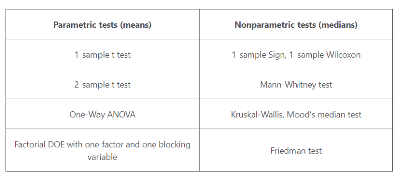
Table below displays various tests, I have verified that all of these tests are available in python stats package.
When to Use Parametric Tests
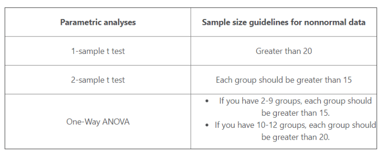
Parametric tests can perform well with skewed and nonnormal distributions
It is important to follow guidance in the sample size of data as shown in table below
Parametric tests can perform well when the spread/variance of each group is different
It has Statistical power
Reasons to Use Nonparametric Tests
Your area of study is better represented by the median
Income distribution is skewed and median is more useful than mean
Few billionaires can boost up the mean significantly
You have a very small sample size
Even less than what is mentioned in table above
You have ordinal data, ranked data, or outliers that you can’t remove
Σ being a positive definite ensure quadratic bowl is downwards
σ2 also being positive ensure that parabola is downwards
On Covariance Matrix
Definition of covariance between two vectors:
When we have more than two variable we present them in matrix form. So covariance matrix will look like
Above is very similar to how we compute sigma^2 in 1-D = (x – mu)^2
Formula of multivariate gaussian distribution demands Σ to be singular and symmetric positive semidefinite, which in terms means sigma will be symmetric positive semidefinite.
For some data above demands might not meet
Side Note
Covariance is directional measure
Correlation is scaled measure
We normalise by individual variance
Derivations
Following derivations are available at [0]:
We can prove[0] that when covariance matrix is diagonal (i.e there is variables are independent) multivariate gaussian distribution is simply multiplication of single gaussian distribution of each variable.
It was derived that shape of isocontours (figure 1) is elliptical and axis length is proportional to individual variance of that variable
Above is true even when covariance matrix is not diagonal and for dimension n>2 (ellipsoids)
First part above says that bi-variant destitution can be generated from two standard normal distribution z = N(0,1).
For any given k-variant Gaussian we can represent it as linear combination of k standard normal distribution. One simpler way to find these coefficient is Cholesky decomposition. Theorem 1 below stats the same thing.
This has a reference from [1].
Linear Transformation Interpretation
This was proved in two steps [0]:
Step-1 : Factorizing covariance matrix
Step-2 : Change of variables, which we apply to density function
On Practical Example
Height, wight and waist size of men in US (Of course it weight can be negative, so it is approximately normal)
Understanding probability rules and solving tricky probability questions can be challenging. In this blog post, we will explore key probability rules and discuss solutions to some intriguing questions.
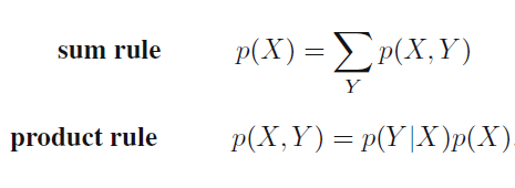
Probability Rules:
Joint Distribution: The probability of events X and Y occurring together is denoted as p(X, Y) and is known as the joint distribution.
Conditional Distribution: The probability of event X given event Y is denoted as p(X/Y) and is known as the conditional distribution.
Marginal Distribution: The probability of event X, with event Y marginalized out, is denoted as p(X) and is known as the marginal distribution.
Operations:
Making Conditional Distribution: To obtain the conditional distribution, normalization is required.
Marginalization: Marginalization does not require normalization.
Note: It is not possible to derive the conditional distribution from the joint distribution solely through integration. There is no direct relationship between them.
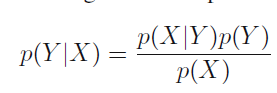
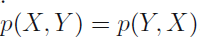
There are just two rules for probability. Sum rule and product rules. And then there is Bayes theorem. Bayes theorem can be derived from product rule and the fact that P(x,y) = P(y,x)
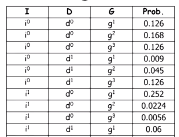
We might want to look at a table like below and calculate joint and conditional distribution and marginalized out one of the variable. [1]
Probability Tricky Question
This questions are taken from [2]. One key to solve this question is write down the sample space and keep eliminating choices. Don’t conclude in hurry.
Q1 : A man comes up to you on the street and says: I have two children. At least one of them is a boy. What is the probability that the other child is also a boy?
Q2 : I have two kids, what are the odds I have 2 boys?
Q3 : A man comes up to you on the street and says: I have two children. The older one is a boy. What is the probability that the other child is also a boy?
Q4 : A man comes up to you on the street and says: I have two children. One is the boy standing here next to me. What is the probability that the other child is also a boy?
Q5 : Q. A man comes up to you on the street and says: I have two children. One of them is a boy who was born in the summer. What is the probability that the other child is also a boy? (There are four seasons : spring, summer, fall, winter)[0]
Ans1 : (1/3)
P(BG) is 1/2 and p(BB) = 1/4 in the universe
Ans2 : (1/4)
Ans3 : (1/2)
Ans4 : (1/2)
Ans5 : (7/15) [0]
Compare Q1 and Q5. Odd increases. Being born in summer is rare thing. If that rare thing has occurred there are higher chances of having two boys.
A bag contains (x) one rupee coins and (y) 50 paise coins. Four coins are taken from the bag and put away. If a coin is now taken at random from the bag, what is the probability that it is a one rupee coin?
Ans is x/(x+y). It will remain same if we take either 1/2/3/4/5 coins because we don’t know which coin has been withdrawn. It is like trying out all possibilities and when we sum, it would come out as 1 only. [4]
The probability of a car passing a certain intersection in a 20 minute windows is 0.9. What is the probability of a car passing the intersection in a 5 minute window? (Assuming a constant probability throughout)
Ans : 0.4377 [5]
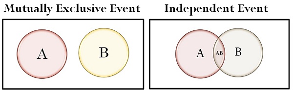
Independent Events
Mutually exclusive events means dependent event
For independent event = P(A/B) = P(A)
For mutually exclusive event if we know B has occurred, A will never occur.
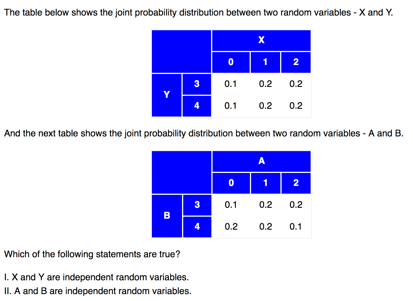
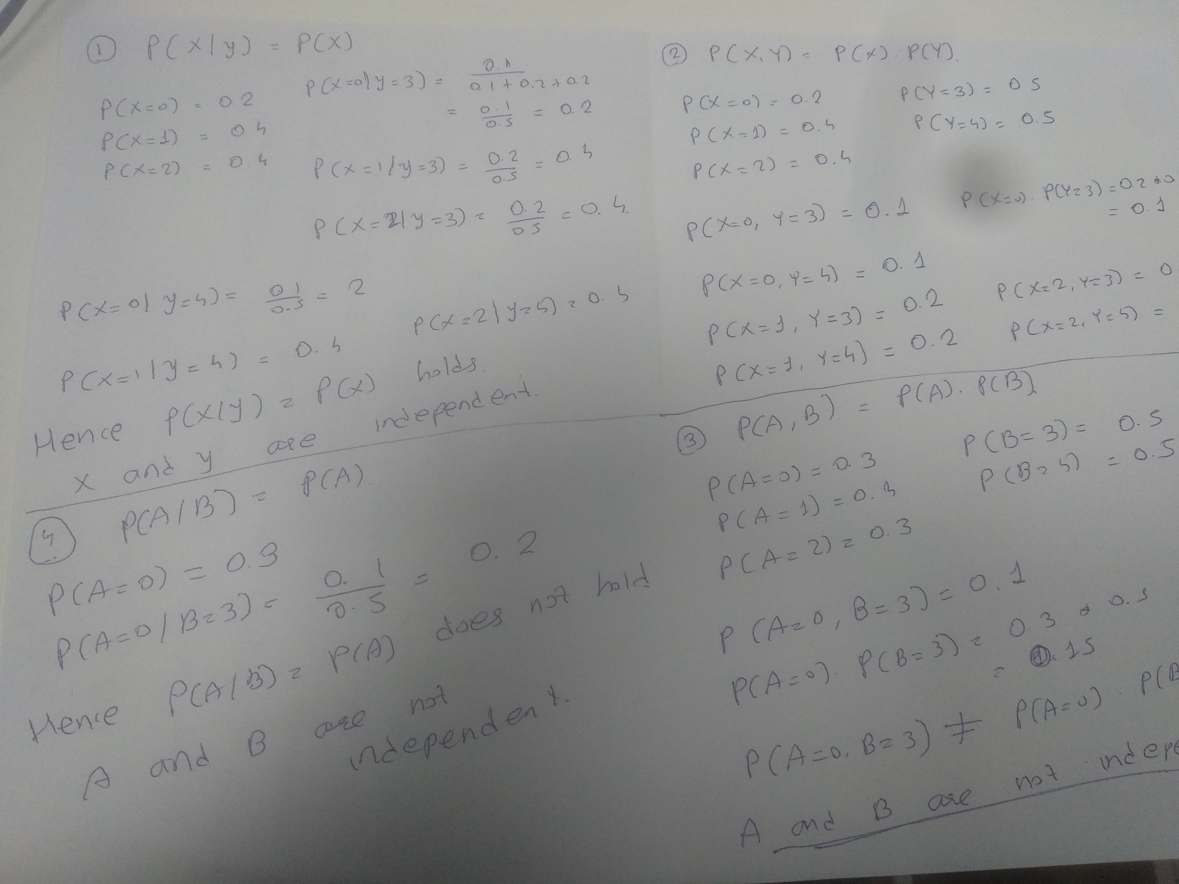
If two random variables, X and Y, are independent, they satisfy the following conditions.
P(x|y) = P(x), for all values of X and Y.
P(X, Y) = P(x ∩ y) = P(x) * P(y), for all values of X and Y.
Here is an example from [6]. Ans is that X and Y are independent, A and B are not.
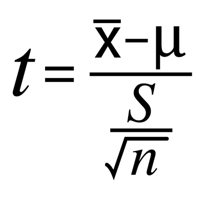
We calculate the t-score using hypothesis data, which also provides us with the degrees of freedom. This value is then supplied to a function that gives us the probability of the hypothesis being true.
The t-test can be seen as a ratio, similar to a signal-to-noise ratio. The numerator allows us to center it around zero, while the denominator represents the standard error of the mean (SEM) calculated as s/sqrt(n), where s is the standard deviation of the samples.
The t-score indicates how many SEM the current mean is away from the mean given in the hypothesis. If it is far away, it suggests a low probability of the null-hypothesis-mean being true, leading us to reject the null hypothesis.
In engineering, we typically assume that the mean and standard deviation are given and true, and we compute the probability of observing the sample. However, in hypothesis testing with a small number of samples, we are testing whether the given mean is true or not.
To address this, we need a distribution that adjusts itself based on the number of observations, widening when there are fewer samples. The t-distribution serves this purpose, as it is dependent on the sample size.
There are different types of t-tests:
One-sample t-test: Compares the mean of a sample with a known population mean.
Discussion so far is for one sample test
Two-sample t-test: Compares the means of two independent groups.
To compare means of two independent groups
Scores of student who get 8 hour sleep vs four hour sleep
Question we want to answer is are there any significant difference in there scores?
In one sample test (In numerator of t-score) we are comparing sample mean with population mean
In two sample test it compares means of two independently drawn sample
And in denominator as well SEM formula is modified
Example
A/B testing on e-commerce site where you compare CTR before and after
This is two sample because you don’t have standard value of CTR before the feature
Even you will see some difference in AA test
Paired t-test: Compares the means of two conditions using the same samples.
This is essentially a one-sample t-test on the differences between values at two conditions.
Same samples are used in two different conditions
10 people before medication and same 10 people after medication
We want to check if medication has any effect
Different time points are used for market calculation
This essentially is a one sample T-test on the differences of value at two different conditions
Example
Interleaving test in e-commence search system
For each search page you will assign some score to control and variant
One-sided t-test: Tests a hypothesis in one direction (e.g., weight of dairy milk is less than 100g).
Two-sided t-test: Tests a hypothesis in both directions (e.g., weight of dairy milk is not equal to 100g).
P-values represent the probability of finding the observed or more extreme results when the null hypothesis is true. It is described in terms of rejecting the null hypothesis when it is actually true, but it is not a direct probability of this state.
For further examples and details, you can refer to the following link: Example Link
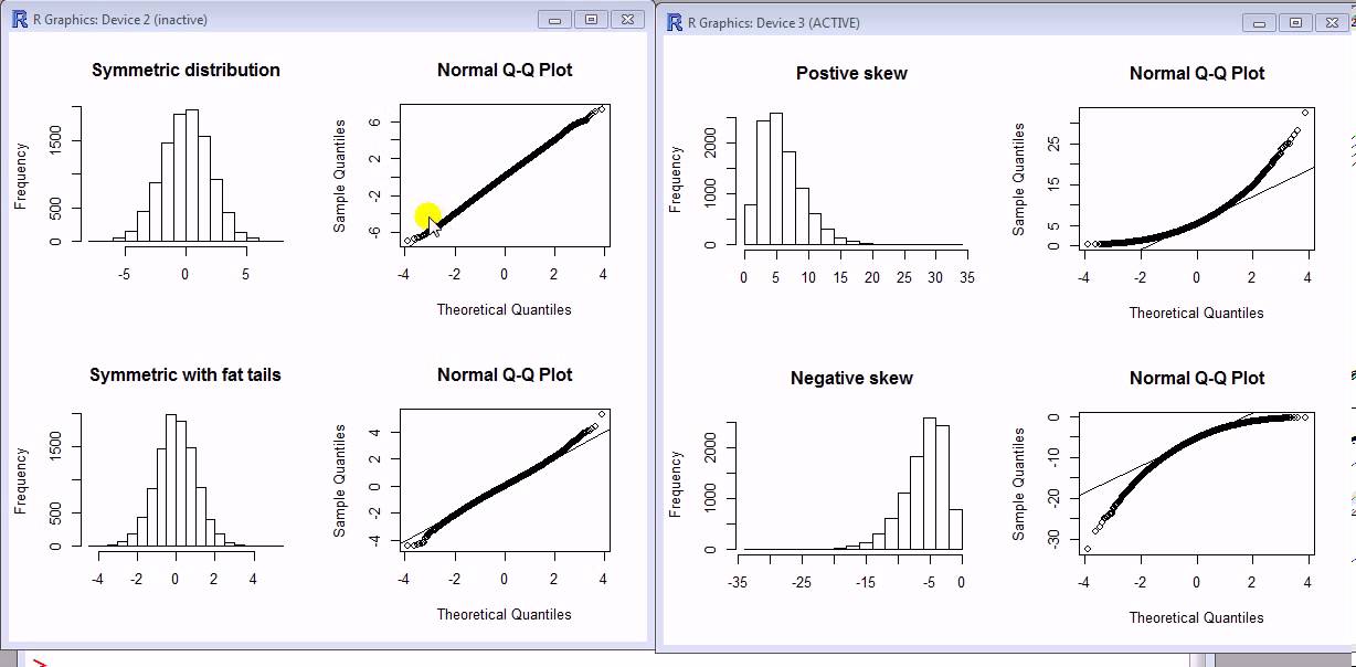
Since few days I was coming across to Q-Q plots very often and thought to learn more about it.
Full form is Quartile-Quantile plot.
Many a times we want our data to be normal, this is because we normality is an assumption behind many statistical models. Now how to test normality. Wikipedia has an article about this which lists many method, one of them is Q-Q plots.
Here is how to create Q-Q plot manually (This steps will show the theory behind it):
Sort your samples (Call it Y). Let n be no of sample. n = len(Y)
Find n values(quartiles) from standard normal distribution to divide it in (n+1) equal areas
Standard normal distribution is a distribution with mean = 0 and standard deviation = 1
Call above X
Plot Y against X
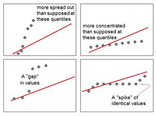
For normal distribution it would be approximately straight line
However considering probability, outliers and no of smaples have role to play
We have learned various probability distribution during high school and engineering courses. However at times we forget them, so here I am providing simple practical scenarios for each distribution with no theories involved.
Bernoulli Distribution
When the random variable has just two outcomes
Probability of Drug/Medicine will be approved by government is p = 0.65
Probability that it will not approve is 0.35
Below formula works when we have probability available, in real life we estimate them from data :
Mean = p
Variance (Sigma Square) = p*(1-p)
Parameters : p
Probability evaluation P(x|params) = p if x = 1, (1-p) if x = 0
MLE : p = n/N, where n = no of time 1 observed , N = no of experiments
MLE = Maximum Likelihood Estimation
Binomial Distribution
When you perform the Bernoulli experiment multiple times and want to see how many times certain outcome appears.
For example you flip a coin(fair/biased) 10 time and probability that head will appear for x (1, 2, …..10) times.
Another more practical example :
Suppose oil price can increase by 3 bucks or decreased by 1 buck each day
Probability of increasing p = 0.65, and that of decreasing = 0.35
What price can we expect after three days
Note (Increase, Increase, Decrease) and (Increase, Decrease, Increase) will give same price.
(2,1) success -> 2 success 1 failure
From another point of view it count no of successes in an experiment :
No of patient responding to treatment
Binary classification problem (Does not seem correct now, it should be Bernoulli, we take logit and sigmoid)
Below formula works when we have probability available, in real life we estimate them from data :
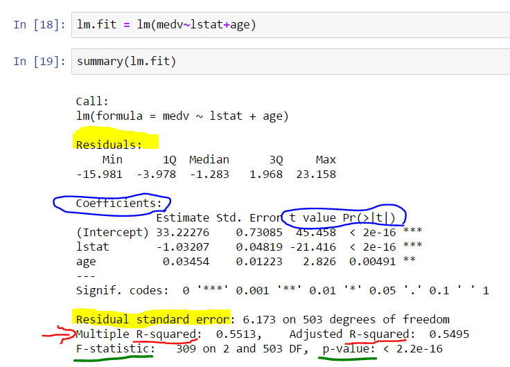
In this post, we will explore the values in the summary(model) output in R and understand their significance.
Here is a screenshot illustrating the summary:
Significance of Residue
We desire our residues to be normally distributed and centered around zero.
It’s similar to aiming at the bullseye on a dartboard.
If the residues are biased in one direction, there is room for improvement.
If the residues are equally biased in all directions, we can attempt to reduce the standard deviation.
Irreducible error should be observed in all directions simultaneously.
Residues quantile provides an initial insight into symmetry.
R also provides the standard deviation of residuals, known as RSE (residue standard error).
The Relationship between t-value and p-value in the Coefficient Section
The values test if a variable has a relationship with the output.
This is a preset statistical question (null hypothesis) that cannot be changed.
If the coefficient is zero, it does not contribute; otherwise, it does.
The t-value indicates the number of standard deviations the mean is away from zero.
A larger t-value signifies a more significant variable.
Calculating p-values
Incorrect thinking: Taking samples from a larger population.
Each sample yields a different coefficient, which can be zero for some samples.
The variance of the estimated parameter can be mathematically derived using (X^T * X)-1 with σ2.
σ2 can be obtained from the residue error.
Bayesian view helps appreciate the distribution of coefficients rather than point estimation.
P-values can be calculated naturally using the T-distribution, as there are no assumptions.
In the R result display, we have a mean and standard deviation.
The coefficient is a probabilistic variable centered at the mean (Estimate in R summary).
The mean is t standard deviations away from zero.
The p-value represents the probability of observing a coefficient beyond t standard deviations from the mean.
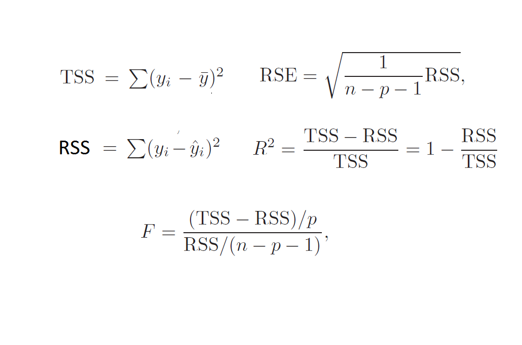
Role of R^2
R^2 indicates how much of the variance is explained by the model. Refer to formulas above for a better understanding.
R^2 has an advantage over RSE as it always falls between 0 and 1.
Determining a Good Value of R^2
A good value of R^2 depends on the problem setting.
When we make perfect predictions, RSS = 0 and hence R^2 = 1
In physics, if we are confident the data follows a linear model, R^2 close to 1 is desirable.
In marketing, a small proportion of the variance can be explained by predictors, so R^2 = 0.1 can be realistic.
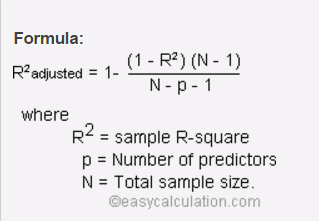
Difference between Absolute and Adjusted R^2
R^2 always increases with the number of variables, while adjusted R^2 decreases if the added variable is not significant.
The formula of adjusted R^2 incorporates the number of variables, so when a non-significant variable is added, the result decreases.
The formulas below illustrate that RSE may increase while RSS decreases, but they are not directly related to R^2.
Significance of F Statistics
The F-test determines if a group of variables is jointly significant, whereas the t-test examines the significance of individual variables.
F-statistics also have associated p-values.
The null hypothesis for the F-test is that the intercept-only model and your model are equal.
While R-squared provides an estimate of the relationship strength between the model and response variable, it does not offer a formal hypothesis test. This test is provided by the F-test.
Why Use F Statistics when Individual Coefficient p-values are Available?
It may seem that if one coefficient is significant (good p-value), the overall model will also be significant.
However, this assumption breaks down when the number of variables with poor p-values is large.
Determining Good Values of F-statistics
It depends on the values of n (number of observations in the training set) and p (number of independent variables).
When n is large, an F-value slightly greater than 1 is sufficient to reject the null hypothesis.
It is advisable to base decisions on corresponding p-values, which consider both n and p.
Degrees of Freedom:
Suppose you have two features, x1 and x2, and a target variable y.
The line equation is y = a1x1 + a2x2 + a3.
In a 3D space, three points define a unique line.
With n points, p(2) features, and 1 target, three points will always lie on the line, while (n-p-1) points can deviate from it. This difference represents the degrees of freedom.
Degrees of freedom are the difference between n and the number of non-zero coefficients, including the intercept.
Significance Score “***” in the Coefficient Section
R indicates the significance of a p-value by displaying stars.
The calculation of this value is likely done through bootstrapping.
Bootstrapping allows assigning measures of accuracy to sample estimates, such as bias, variance, confidence intervals, or prediction error.
In Bayesian inference, parameter distributions are obtained, allowing the calculation of p-values.