Q – Q Plots

update :

Q-Q plots can be used to test goodness of fit for any distribution. There are p-p plots and other method as well.

https://stats.stackexchange.com/questions/132652/how-to-determine-which-distribution-fits-my-data-best

There is also a P-P plot.

https://en.wikipedia.org/wiki/P%E2%80%93P_plot


Since few days I was coming across to Q-Q plots very often and thought to learn more about it.

Full form is Quartile-Quantile plot.

Many a times we want our data to be normal, this is because we normality is an assumption behind many statistical models. Now how to test normality. Wikipedia has an article about this which lists many method, one of them is Q-Q plots.

Here is how to create Q-Q plot manually (This steps will show the theory behind it):

  1. Sort your samples (Call it Y). Let n be no of sample. n = len(Y)
  2. Find n values(quartiles) from standard normal distribution to divide it in (n+1) equal areas
    1. Standard normal distribution is a distribution with mean = 0 and standard deviation = 1
  3. Call above X
  4. Plot Y against X
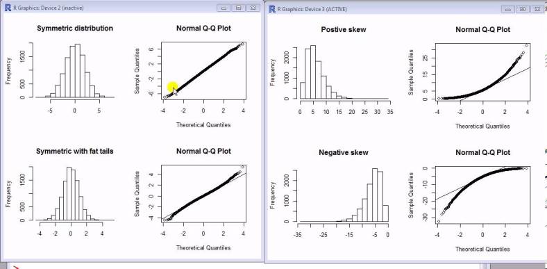
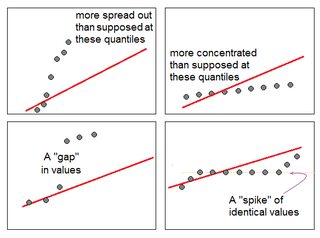
  5. For normal distribution it would be approximately straight line
    1. However considering probability, outliers and no of smaples have role to play

Here is the example code and plots in pythons:

maxresdefaultSnLhAm

Reference :

  1. You tube video 

Probability Distribution

We have learned various probability distribution during high school and  engineering courses. However at times we forget them, so here I am providing simple practical scenarios for each distribution with no theories involved.

Bernoulli Distribution

  • When the random variable has just two outcomes
  • Probability of Drug/Medicine will be approved by government is p = 0.65
    • Probability that it will not approve is 0.35
  • Below formula works when we have probability available, in real life we estimate them from data :
    • Mean = p
    • Variance (Sigma Square) = p*(1-p)
  • Parameters : p
  • Probability evaluation P(x|params) = p if x = 1, (1-p) if x = 0
  • MLE : p = n/N, where n = no of time 1 observed , N = no of experiments
  • MLE = Maximum Likelihood Estimation

Binomial Distribution

  • When you perform the Bernoulli experiment multiple times and want to see how many times certain outcome appears.
  • For example you flip a coin(fair/biased) 10 time and probability that head will appear for x (1, 2, …..10) times.
  • Another more practical example :
    • Suppose oil price can increase by 3 bucks or decreased by 1 buck each day
    • Probability of increasing p = 0.65, and that of decreasing = 0.35
    • What price can we expect after three days
    • Note (Increase, Increase, Decrease) and (Increase, Decrease, Increase) will give same price.
      • (2,1) success -> 2 success 1 failure
  • From another point of view it count no of successes in an experiment :
    • No of patient responding to treatment
    • Binary classification problem (Does not seem correct now, it should be Bernoulli, we take logit and sigmoid)
  • Below formula works when we have probability available, in real life we estimate them from data :
    • n = no of times experience is performed
    • Mean = n*p
    • Variance (Sigma Square) = n*p*(1-p)
  • Example of binomial used in modeling :
  • Parameters : n, p
  • Probability evaluation P(x|params) = nCx * p^x * (1-p)^(1-x)
  • MLE
    • n = no of samples = N
    • p = n/N where n = no of successes
    • Interestingly MLE for binomial and multinomial distribution is very simple

Continue reading “Probability Distribution” →

Interpreting Statistical Values

In this post, we will explore the values in the summary(model) output in R and understand their significance.

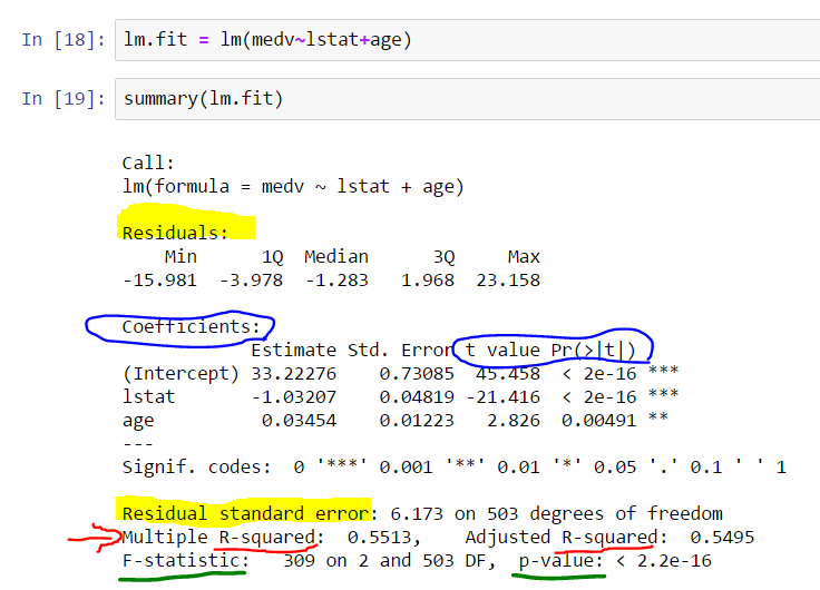
Here is a screenshot illustrating the summary:

rsummary

Significance of Residue

  • We desire our residues to be normally distributed and centered around zero.
  • It’s similar to aiming at the bullseye on a dartboard.
    • If the residues are biased in one direction, there is room for improvement.
    • If the residues are equally biased in all directions, we can attempt to reduce the standard deviation.
    • Irreducible error should be observed in all directions simultaneously.
  • Residues quantile provides an initial insight into symmetry.
  • R also provides the standard deviation of residuals, known as RSE (residue standard error).

The Relationship between t-value and p-value in the Coefficient Section

  • The values test if a variable has a relationship with the output.
  • This is a preset statistical question (null hypothesis) that cannot be changed.
  • If the coefficient is zero, it does not contribute; otherwise, it does.
  • The t-value indicates the number of standard deviations the mean is away from zero.
  • A larger t-value signifies a more significant variable.

Calculating p-values

  • Incorrect thinking: Taking samples from a larger population.
  • Each sample yields a different coefficient, which can be zero for some samples.
  • The variance of the estimated parameter can be mathematically derived using (X^T * X)-1 with σ2.
  • σ2 can be obtained from the residue error.
  • Bayesian view helps appreciate the distribution of coefficients rather than point estimation.
    • P-values can be calculated naturally using the T-distribution, as there are no assumptions.
  • In the R result display, we have a mean and standard deviation.
    • The coefficient is a probabilistic variable centered at the mean (Estimate in R summary).
    • The mean is t standard deviations away from zero.
    • The p-value represents the probability of observing a coefficient beyond t standard deviations from the mean.

formulas

Role of R^2

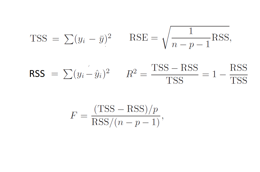
  • R^2 indicates how much of the variance is explained by the model. Refer to formulas above for a better understanding.
  • R^2 has an advantage over RSE as it always falls between 0 and 1.

Determining a Good Value of R^2

  • A good value of R^2 depends on the problem setting.
  • When we make perfect predictions, RSS = 0 and hence R^2 = 1
  • In physics, if we are confident the data follows a linear model, R^2 close to 1 is desirable.
  • In marketing, a small proportion of the variance can be explained by predictors, so R^2 = 0.1 can be realistic.

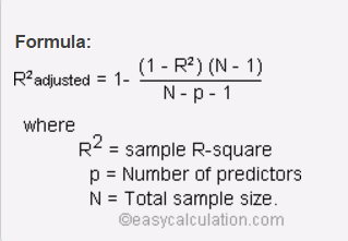
Difference between Absolute and Adjusted R^2

  • R^2 always increases with the number of variables, while adjusted R^2 decreases if the added variable is not significant.
  • The formula of adjusted R^2 incorporates the number of variables, so when a non-significant variable is added, the result decreases.
  • The formulas below illustrate that RSE may increase while RSS decreases, but they are not directly related to R^2.
adR2.PNG

Significance of F Statistics

  • The F-test determines if a group of variables is jointly significant, whereas the t-test examines the significance of individual variables.
  • F-statistics also have associated p-values.
  • The null hypothesis for the F-test is that the intercept-only model and your model are equal.
  • While R-squared provides an estimate of the relationship strength between the model and response variable, it does not offer a formal hypothesis test. This test is provided by the F-test.

Why Use F Statistics when Individual Coefficient p-values are Available?

  • It may seem that if one coefficient is significant (good p-value), the overall model will also be significant.
  • However, this assumption breaks down when the number of variables with poor p-values is large.

Determining Good Values of F-statistics

  • It depends on the values of n (number of observations in the training set) and p (number of independent variables).
  • When n is large, an F-value slightly greater than 1 is sufficient to reject the null hypothesis.
  • It is advisable to base decisions on corresponding p-values, which consider both n and p.

Degrees of Freedom:

  • Suppose you have two features, x1 and x2, and a target variable y.
  • The line equation is y = a1x1 + a2x2 + a3.
  • In a 3D space, three points define a unique line.
  • With n points, p(2) features, and 1 target, three points will always lie on the line, while (n-p-1) points can deviate from it. This difference represents the degrees of freedom.
  • Degrees of freedom are the difference between n and the number of non-zero coefficients, including the intercept.

Significance Score “***” in the Coefficient Section

  • R indicates the significance of a p-value by displaying stars.
  • The calculation of this value is likely done through bootstrapping.
  • Bootstrapping allows assigning measures of accuracy to sample estimates, such as bias, variance, confidence intervals, or prediction error.
  • In Bayesian inference, parameter distributions are obtained, allowing the calculation of p-values.

References

Found the formula for adjusted R2 here